Method 1 -Using COUNT Function to Count Cell Numbers
The syntax for the COUNT function is:
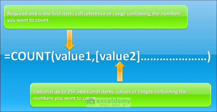
Steps:
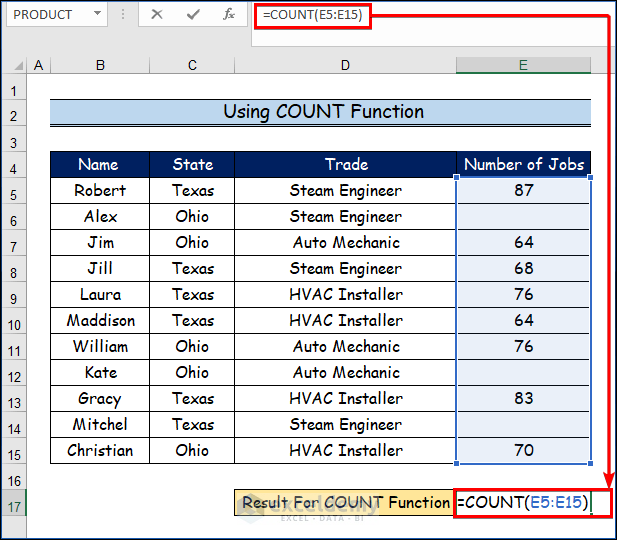
- To count only the number of jobs in the list, select cell E17.
- Enter the following formula.
=COUNT(E5:E15)- Press CTRL+ENTER.
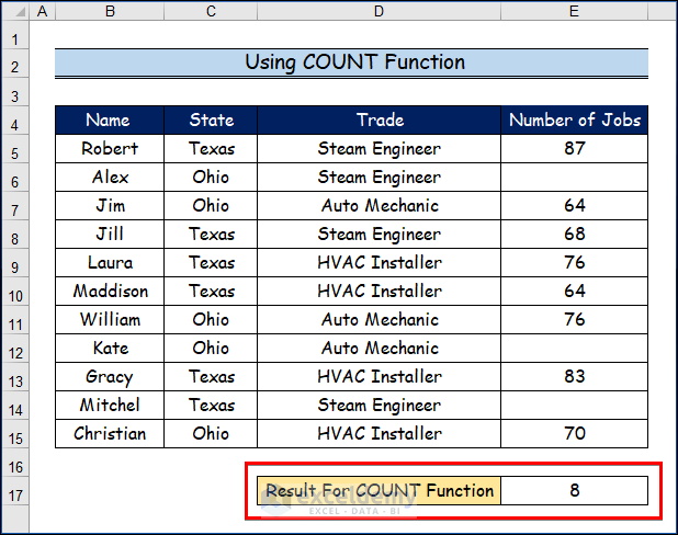
- It will count and display the number of jobs for tradies, which is 8.
Read More: How to Find 5 Most Frequent Numbers in Excel
Method 2 – Utilizing COUNTA Function to Count Cell Texts
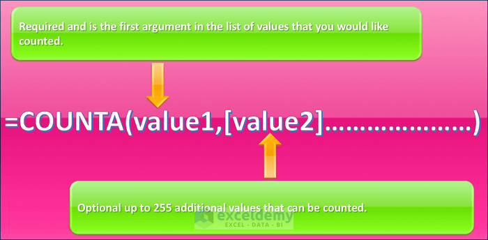
The syntax for the COUNTA function is:
Steps:
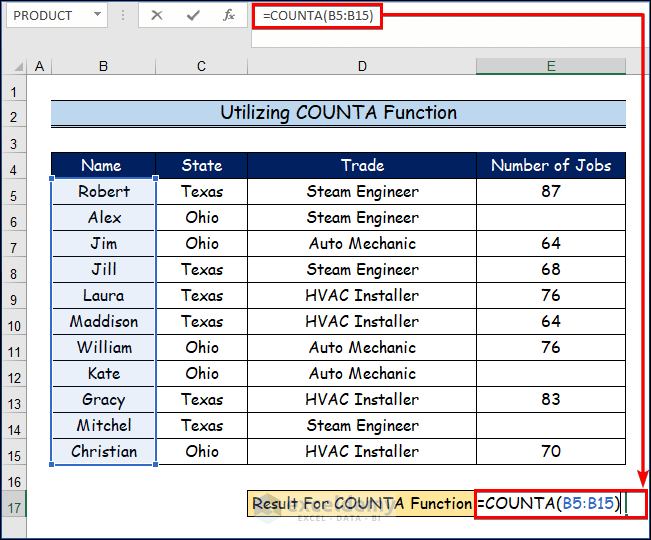
- Enter the following formula in cell E17.
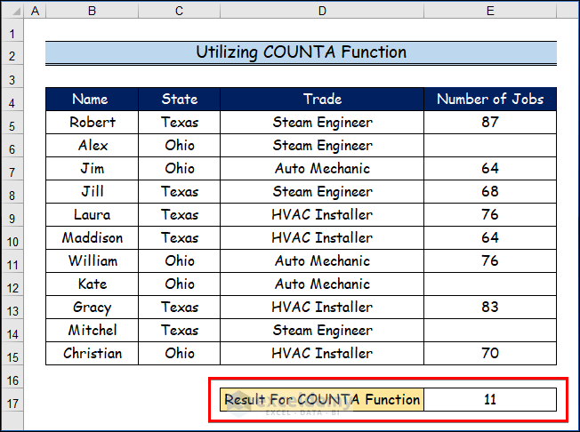
=COUNTA(B5:B15)- Press CTRL+ENTER.
Step 2:
- It will count and display the number of tradies available, which is 11.
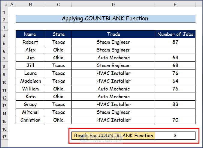
Method 3 – Applying COUNTBLANK Function to Count Blank Cells
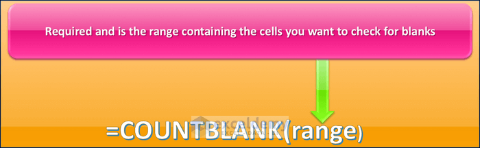
The syntax for the COUNTBLANK function is:
Steps:
- Enter the following formula in Cell E17.
=COUNTBLANK(E5:E15)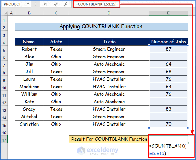
- Press CTRL+ENTER.
- It will count and display the number of blank cells, which is 3.
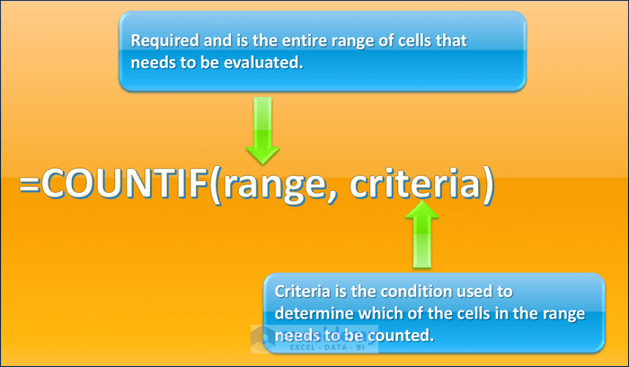
Method 4 – Inserting COUNTIF Function to Count with a Single Criterion
The syntax for the COUNTIF function is:
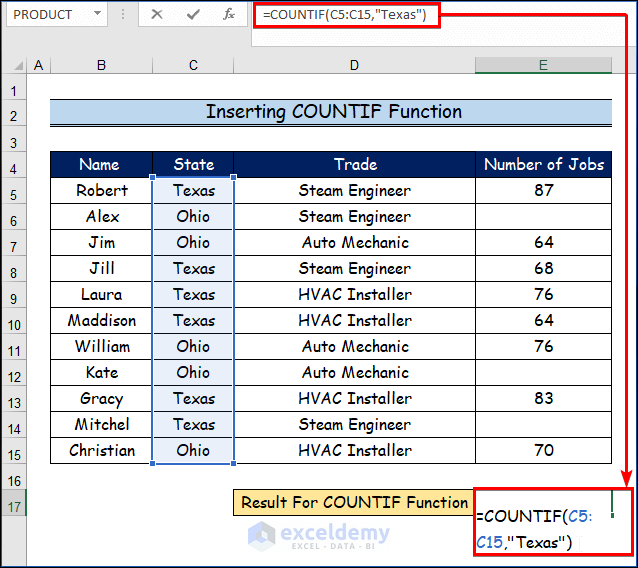
Steps:
- To count how many tradies work in Texas, enter the following formula in cell E17.
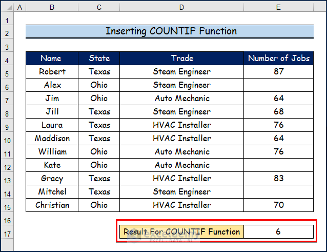
=COUNTIF(C5:C15, "Texas")- Press CTRL+ENTER.
- It will count and display the number of tradies working in Texas, which is 6.
Read More: [Fixed] Excel COUNT Function Not Working
Method 5 – Using COUNTIFS Function to Count with Multiple Conditions
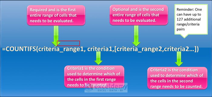
The COUNTIFS function is similar to the COUNTIF function, except it’s used to count the number of cells in a range that meet multiple criteria. The syntax for the COUNTIFS function is:
Steps:
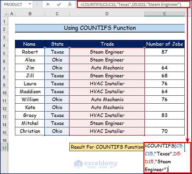
- To count the number of tradies in Texas who are Steam Engineers, apply the formula below in cell E17.
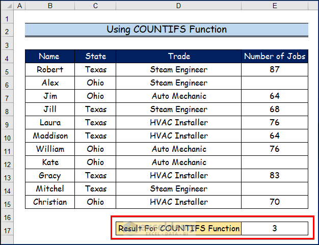
=COUNTIFS(C5:C15,"Texas",D5:D15,"Steam Engineer")- Press CTRL+ENTER.
- It will count and display the number of tradies in Texas who are steam engineers, which is 3.
Download Practice Workbook
<< Go Back to Excel COUNT Function | Excel Functions | Learn Excel
Get FREE Advanced Excel Exercises with Solutions!
