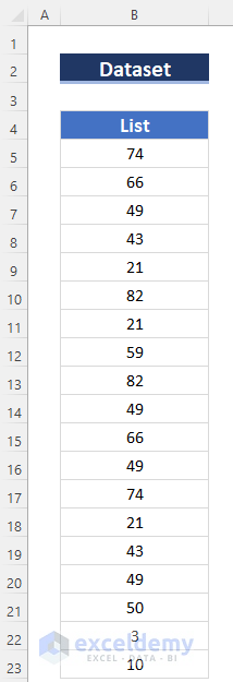
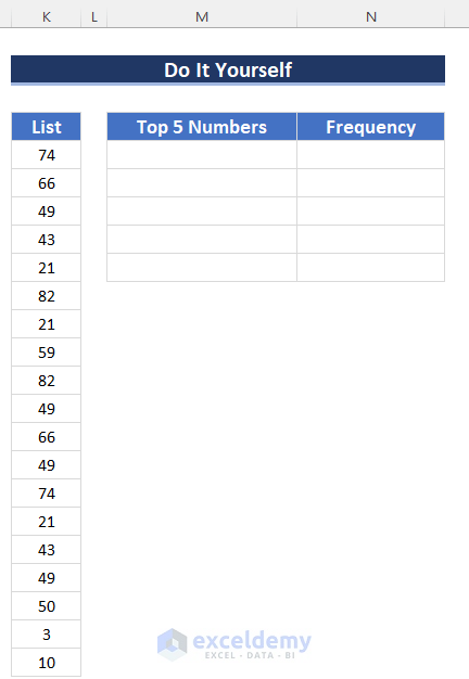
How to Find the 5 Most Frequent Numbers in Excel (4 Methods)

Dataset Overview

To demonstrate the 4 methods, we’ll use a list of 19 numbers.

Dataset for how to Find 5 Most Frequent Numbers in Excel

Method 1 – Using Excel MODE, IF, ISERROR, and MATCH Functions

Steps

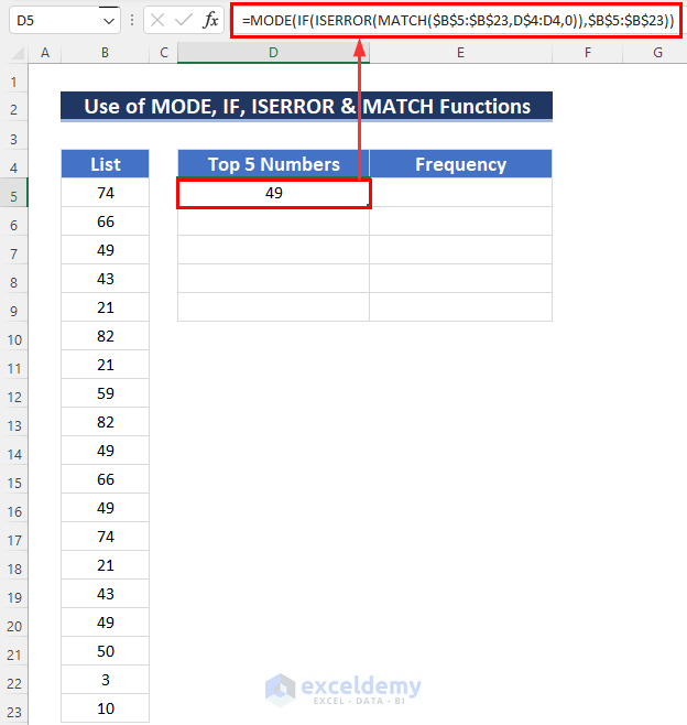
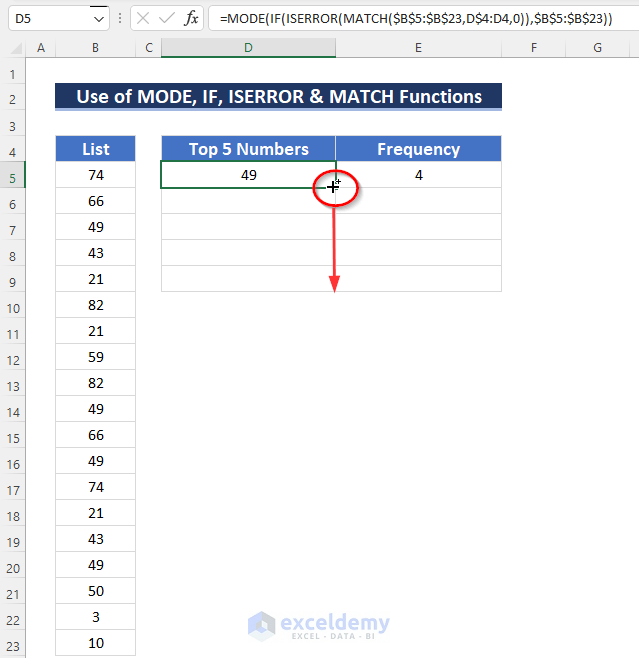
In cell D5, enter the following Excel formula:

=MODE(IF(ISERROR(MATCH($B$5:$B$23,D$4:D4,0)),$B$5:$B$23))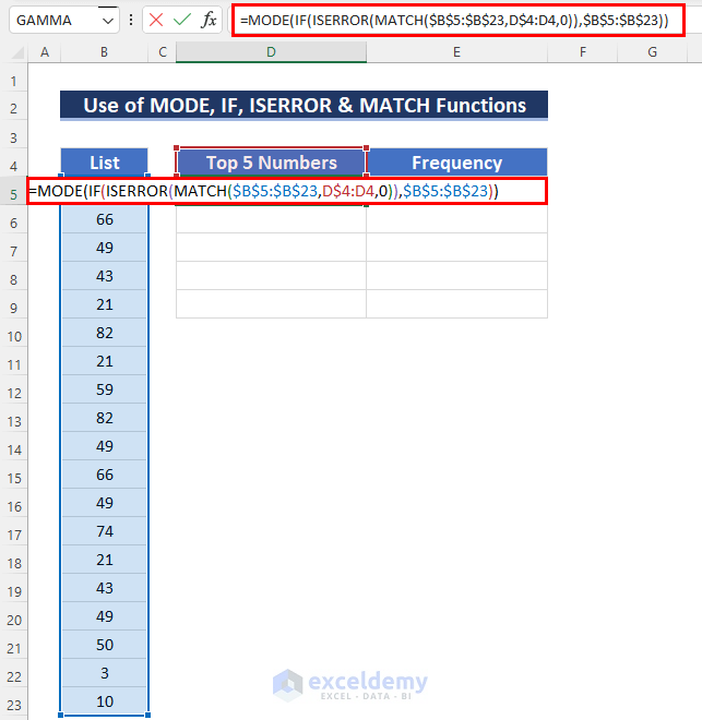

Press ENTER to get the result and the result, which is 49.

Note: If you’re using an older version of Excel than Office 365, enter this formula as an array formula by pressing CTRL+SHIFT+ENTER simultaneously.

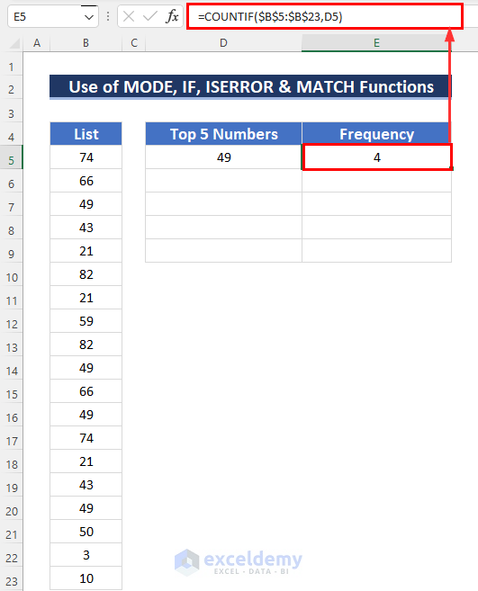
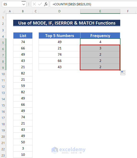
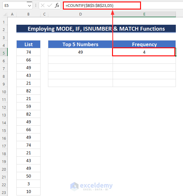
To show the frequency of the number in the list, use the Excel COUNTIF function. In cell E5, enter:

=COUNTIF($B$5:$B$23,D5)

Here, the COUNTIF function finds the frequency. The COUNTIF function will return the total cell numbers within the $B$5:$B$23 range which will contain the value of the D5 cell.

Press ENTER.

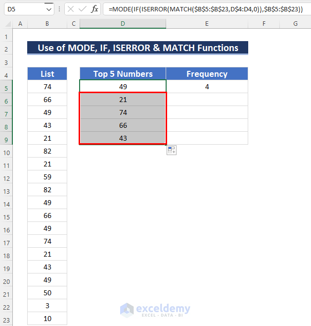
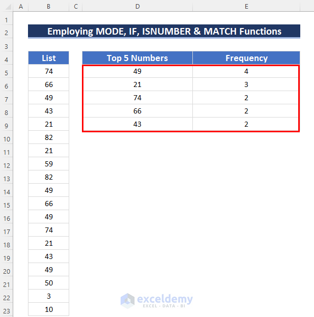
Apply the formula from cell D5 (for finding the 5 most frequent numbers) to other cells in the column using Excel’s Fill Handle Tool.

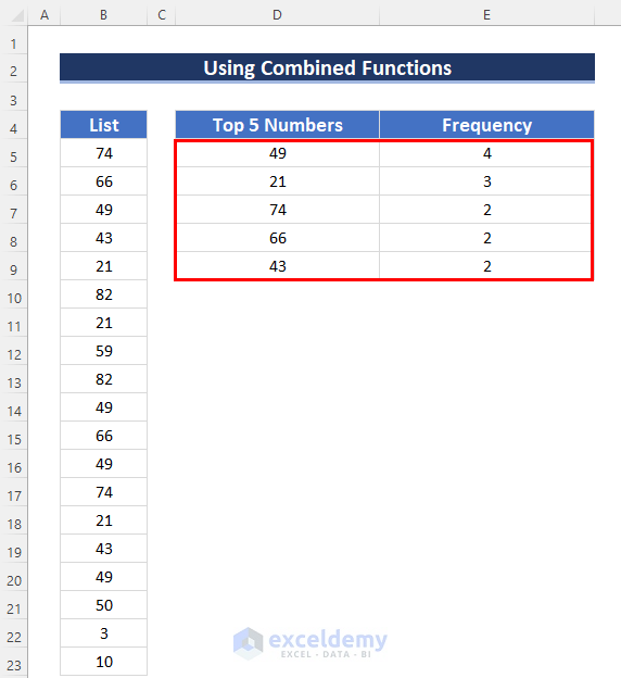
The 5 most frequent numbers will be displayed.

Copy the formula from cell E5 (for counting frequencies) using relative cell references. To do this, drag the Fill Handle icon down to cell E9 and release the mouse button.

You’ll now see the 5 most frequent numbers along with their frequencies.

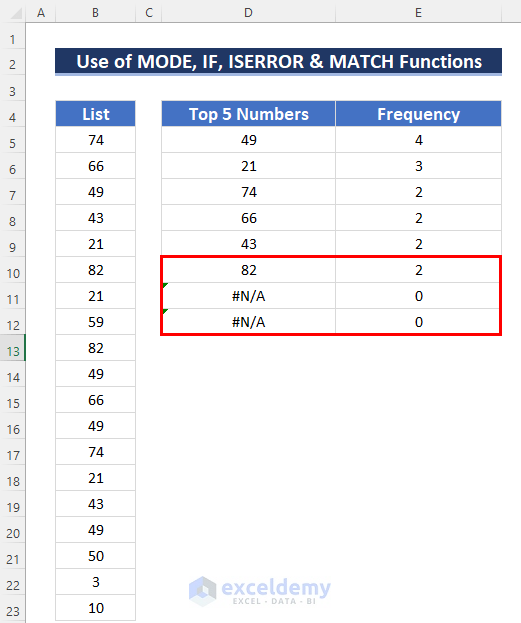
Note: If you want to find more than the 5 most frequent numbers, continue dragging the mouse pointer. The last two cells may display an Excel error value (#N/A) because the MODE function doesn’t find numbers with a frequency greater than 1.

A step-by-step explanation on how this Excel formula works is given below:

Formula Breakdown

The formula in the cell D5:

The MATCH function compares the values in the range $B$5:$B$23 with the partial lookup array D$4:D4.
Since there’s no match, it returns an array of #N/A errors.
The ISERROR function then converts these errors to TRUE values.
The IF function evaluates each TRUE value and returns the corresponding number from the list.
The MODE function calculates the most frequent number from the resulting array, which is 49.
This is the returned value by the MATCH part: MATCH($B$5:$B$23,D$4:D4,0)

The formula in the cell D6:

The lookup array changes to D$4:D5 (relative to the previous cell).
The MATCH function now finds 49 at position 2 in the lookup array.
The ISERROR function converts this position (2) to FALSE.
The IF function returns FALSE for non-error values.
The MODE function considers only numerical values, resulting in 21 (the second most frequent number).

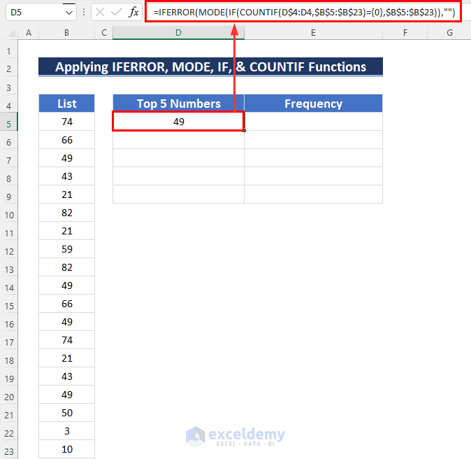
Method 2 – Using IFERROR, MODE, IF, and COUNTIF Functions

Steps

In cell D5, enter the following formula:

=IFERROR(MODE(IF(COUNTIF(D$4:D4,$B$5:$B$23)={0},$B$5:$B$23)),"")

Press ENTER (or CTRL+SHIFT+ENTER for older Excel versions) to get the result.

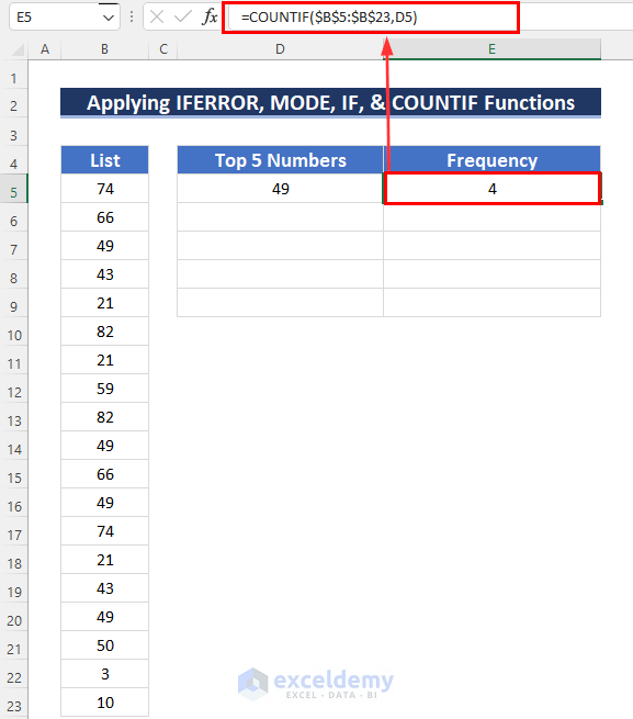
In cell E5, enter this formula to find the frequency:

=COUNTIF($B$5:$B$23,D5)

Press ENTER to get the result.

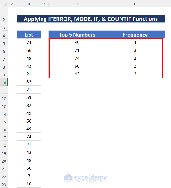
Apply these formulas to the other four cells in the column. The 5 most frequent numbers will be displayed.

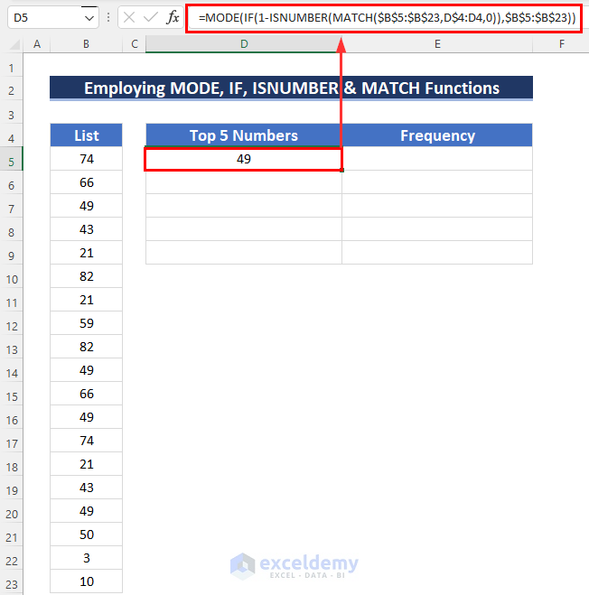
Method 3 – Using MODE, IF, ISNUMBER, and MATCH

In cell D5, enter the following formula:

=MODE(IF(1-ISNUMBER(MATCH($B$5:$B$23,D$4:D4,0)),$B$5:$B$23))

Press ENTER (or CTRL+SHIFT+ENTER for older Excel versions) to get the result.

In cell E5, enter the same COUNTIF formula as before to find the frequency.

=COUNTIF($B$5:$B$23,D5)

Press ENTER to get the result.

Apply these formulas to other cells in the column using the Fill Handle Tool.

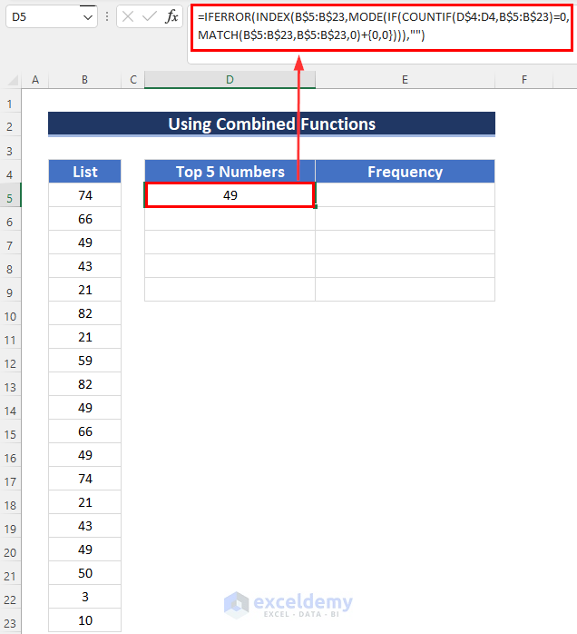
Method 4 – Employing Combined Functions

Click cell D5 to select it.
Enter this formula:

=IFERROR(INDEX(B$5:B$23,MODE(IF(COUNTIF(D$4:D4,B$5:B$23)=0,MATCH(B$5:B$23,B$5:B$23,0)+{0,0}))),"")

Press ENTER (or CTRL+SHIFT+ENTER for older Excel versions) to get the result.

Formula Breakdown

MATCH(B$5:B$23,B$5:B$23,0):

The MATCH function compares each value in the range B$5:B$23 with the same range itself (exact match, indicated by the third argument 0).
Since the range is sequential, it returns an array of positions corresponding to each value:

{1;2;3;4;5;6;7;8;9;10;11;12;13;14;15;16;17;18;19}

COUNTIF(D$4:D4,B$5:B$23):

This formula calculates the count of occurrences of each value in the range B$5:B$23 within the partial lookup array D$4:D4.
Since D$4:D4 contains only one value (D4), the result is an array of zeros:

{0;0;0;0;0;0;0;0;0;0;0;0;0;0;0;0;0}

IF(1-ISNUMBER(MATCH($B$5:$B$23,D$4:D4,0)),$B$5:$B$23):

The IF function checks if the expression 1-ISNUMBER(MATCH($B$5:$B$23,D$4:D4,0)) is TRUE or FALSE for each value in B$5:$B$23.
Since the MATCH result is zero for all values, the expression evaluates to TRUE (1-0=1) for all elements.
Therefore, the IF function returns the entire B$5:$B$23 array:

{74;66;49;43;21;59;82;49;66;49;66;49;74;21;43;49;50;3;10}

MODE(IF(…)):

The MODE function calculates the most frequent number from the array obtained in step 3.
The most frequent number is 49.

INDEX(B$5:B$23,3):

The INDEX function retrieves the value at the third position in the range B$5:B$23.
The third position corresponds to the value 49.

IFERROR(49,“”):

The IFERROR function wraps the result from step 5.
Since there is no error, it simply returns 49.

Now, I will find the frequencies.

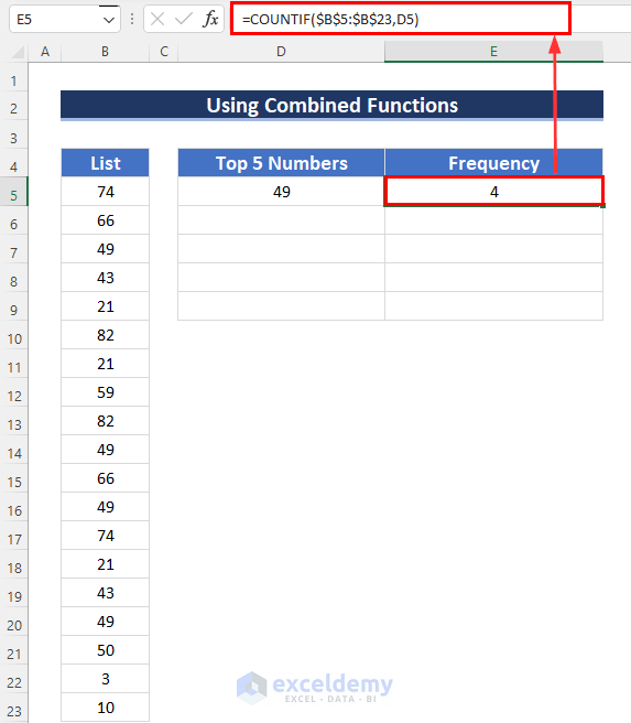
To find the frequencies, enter the same COUNTIF formula in cell E5.

=COUNTIF($B$5:$B$23,D5)

$B$5:$B$23 means the data range and criteria D5 means: the value of cell D5. In one sentence the whole command is: Count in the value if the value is equal to D5 in the data range $B$5:$B$23.

Press ENTER to get the result.

Apply these formulas to other cells in the column using the Fill Handle Tool.

Using of MAX Function to Find the Highest Numbers in Excel

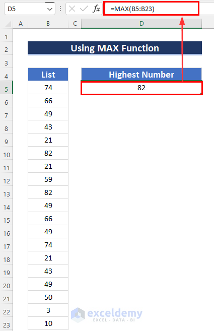
Click on cell D5 to select it.
In that cell, enter the following formula:

=MAX(B5:B23)

Press ENTER to get the result.

This will give you the highest number from the given list. It’s a straightforward way to find the maximum value in Excel.

Finding the 2nd Most Frequent Number by Using MODE & IF Functions in Excel

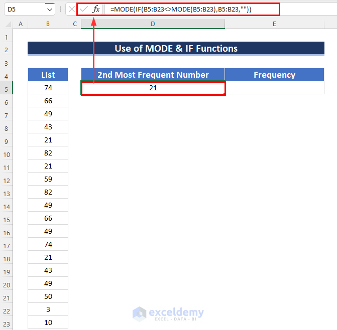
Click on cell D5 to select it.
In that cell, enter this formula:

=MODE(IF(B5:B23<>MODE(B5:B23),B5:B23,""))

Press ENTER to get the result.

Formula Breakdown

The MODE function finds the most frequent number in the array B5:B23 (which turns out to be 49).
The IF function then returns the value that meets the given criteria (not equal to 49).
The resulting array is: {74;66; ;43;21;82;21;59;82; ;66;FALSE;74;21;43; ;50;3;10}.
Since the 1st most frequent number is blank, the MODE function gives us the 2nd most frequent number, which is 21.

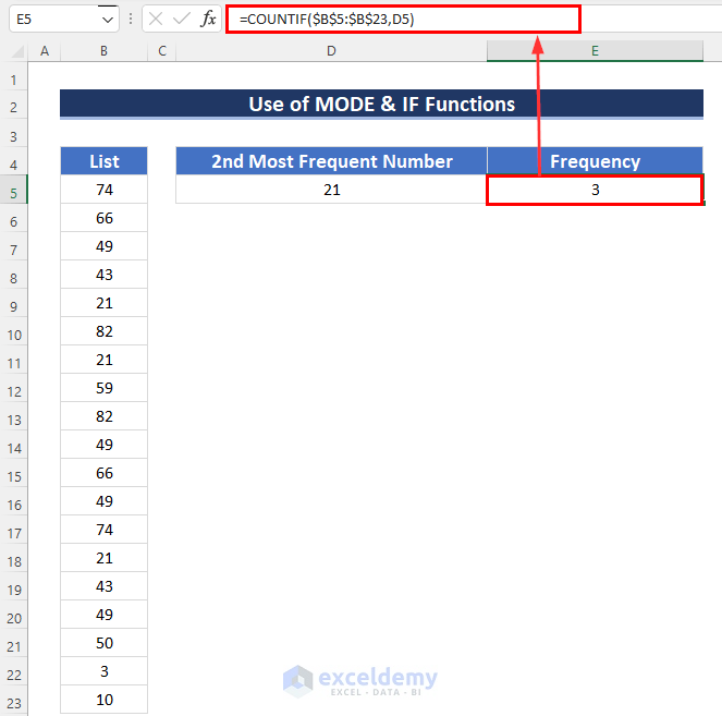
To find the frequencies:

Click on cell E5 to select it.
Enter this formula:

=COUNTIF($B$5:$B$23,D5)

- This counts how many times the value in cell D5 appears in the data range $B$5:$B$23.
Press ENTER to get the frequency of the 2nd most frequent number.

Practice Section

Feel free to practice these steps on your own.

Download Practice Workbook

You can download the practice workbook from here:

Finding Most Frequent Numbers.xlsx

<< Go Back to Formula List | Learn Excel

Get FREE Advanced Excel Exercises with Solutions!

Sub FindTop5FrequentNumbers() Dim dataRange As Range Dim resultRange As Range Dim frequencyRange As Range Dim dict As Object Dim cell As Range Dim i As Integer Dim keyArray As Variant ' Set the range that contains your sample data (E2:I57) Set dataRange = ThisWorkbook.Worksheets("Sheet1").Range("E2:I57") ' Adjust the sheet name and range as per your data ' Set the range where you want to output the top 5 most frequent numbers (M4:M9) Set resultRange = ThisWorkbook.Worksheets("Sheet1").Range("M4:M9") ' Adjust the sheet name and range as per your choice ' Set the range where you want to output the corresponding frequencies (N4:N9) Set frequencyRange = ThisWorkbook.Worksheets("Sheet1").Range("N4:N9") ' Adjust the sheet name and range as per your choice ' Create a dictionary to store the frequencies of each number Set dict = CreateObject("Scripting.Dictionary") ' Loop through each cell in the data range to count the occurrences of each number For Each cell In dataRange If IsNumeric(cell.Value) Then If dict.Exists(cell.Value) Then dict(cell.Value) = dict(cell.Value) + 1 Else dict.Add cell.Value, 1 End If End If Next cell ' Convert the dictionary keys (numbers) to an array keyArray = dict.keys ' Sort the array based on the frequencies in descending order For i = LBound(keyArray) To UBound(keyArray) - 1 For j = i + 1 To UBound(keyArray) If dict(keyArray(j)) > dict(keyArray(i)) Then ' Swap elements temp = keyArray(i) keyArray(i) = keyArray(j) keyArray(j) = temp End If Next j Next i ' Output the top 5 most frequent numbers and their frequencies to the result and frequency ranges For i = 1 To 5 If i <= UBound(keyArray) + 1 Then resultRange.Cells(i, 1).Value = keyArray(i - 1) frequencyRange.Cells(i, 1).Value = dict(keyArray(i - 1)) Else resultRange.Cells(i, 1).Value = "" frequencyRange.Cells(i, 1).Value = "" End If Next i End Sub

18 Comments

Frank May 21, 2019 at 8:10 PM

Thanks a lot this has been a challenge to me for some time now.

Frank
- Reply
  Kawser May 21, 2019 at 9:54 PM
  
  You’re welcome, Frank! Feeling good to hear that this article helped you.
  Best regards
Dennis Paul Eagan Jul 25, 2019 at 5:37 PM

Thank you for this and all your information. I do appreciate it all. Dennis
- Reply
  Kawser Jul 25, 2019 at 6:33 PM
  
  You’re most welcome, Dennis!
  Thanks for the nice words.
  Best regards
  Kawser Ahmed
KKRAO Oct 19, 2019 at 9:07 PM

In the first sight, I did not understand the usage of this formula, Sorry.
Where it is useful, in what contest? If it is finding the numbers, we can sort them in ascending or descending order then we can see the contents of the row.
I request you please enlighten me.
- Reply
  Kawser Feb 17, 2021 at 9:24 PM
  
  Hi Kkrao,
  I understand your thought.
  It is possible for small numbers to count the top ones, but if you have good numbers in a list, you might need an automatic process. And sometimes, you might need the output to feed a system’s input, so I hope you get my point for making a formula for this.
  Thanks.
Wayne Edmondson Oct 29, 2019 at 11:01 AM

Hi Kawser.. excellent. I was aware of one of your methods.. but learned a lot interrogating the other two. Note for users that you can use MODE() .. the older function or MODE.SNGL() .. the newer function. Either works.. but generally I try and use the newer functions to train my brain to go forward. Thanks for sharing all of your knowledge and skills in the blog posts.. very helpful and appreciated. Thumbs up!
- Reply
  Kawser Feb 17, 2021 at 9:23 PM
  
  Wayne,
  Thanks for your feedback.
Evon Aug 10, 2021 at 10:23 PM

Thanks for this. When I use the formula in my sheet, it keeps repeating the result twice. Do you have any idea why this is happening?
- Reply
  Kawser Aug 10, 2021 at 10:39 PM
  
  The best way is, please send the sheet to me at [email protected]
arun Oct 16, 2021 at 2:09 PM

why this formula only picking top 9 numbers only
- Reply
  Tanjim Reza Aug 30, 2022 at 3:15 PM
  
  Hi, ARUN!
  Thank you for your query.
  According to our dataset, we have 9 values that are repeated twice or thrice. Other values are unique and have come only once in the dataset. As the formula is about finding the frequent numbers, it is returning those repeated 9 numbers only.
  
  Regards,
  Tanjim Reza
RC GOYAL Dec 20, 2022 at 6:00 PM

Hi Kawser.. excellent. Thanks for sharing all of your knowledge and skills in the blog posts.. very helpful and appreciated. I could not understand about using of +{0,0} in the last of combined formula.

Thanks dear
- Reply
  Arin Dec 21, 2022 at 12:09 PM
  
  Hi RC GOYAL,
  Thanks for your feedback.
  In the formula, we used {0,0} in the combination formula to return a two column array. However, you can avoid it for this dataset. It will return the same result.
  If you face any further problems, please share your Excel file with us at [email protected].
  Regards
  Arin Islam,
  Exceldemy.
ken Feb 2, 2023 at 5:06 PM

Hi Thank you for explaining the above in detail. This will work if the data is in one column. What if the data is spread across ie col A, B, C and D. Is there a way to work out the 5 most frequent number and also the frequency? thank you Ken
- Reply
  Al Ikram Amit Jul 11, 2023 at 5:01 PM
  Dear KEN,
  
  Thank you for your question. If your data is spread across columns A, B, C, and D, you can still work out the 5 most frequent numbers and their frequencies using Excel formulas. Here’s a step-by-step approach:
  1. Assuming that your data starts from row 5, you can use the following formula in cell F5 to get the 5 most frequent numbers:
  =IFERROR(MODE(IF(COUNTIF(F$4:F4,$A$5:$D$23)={0},$A$5:$A$23)),"")
  1. To calculate the frequency of each of the top 5 most frequent numbers, you can use the following formula in cell G5:
  =COUNTIF($A$5:$D$23,F5)
  1. Copy the formulas down by dragging the fill handle for cells F5:F9 and G5:G9 to get the top 5 most frequent numbers and their frequencies.
  I hope this helps! If you have any further questions, feel free to ask.
  
  Best regards
  
  Al Ikram Amit
  
  Team ExcelDemy
  - Reply
    Gracie Jul 18, 2023 at 5:52 AM
    
    Hi,
    
    I tried your method above with numbers spanning to 5 columns and changed the formula to fit my table: =IFERROR(MODE(IF(COUNTIF(M$4:M4,$E$2:$I$57)={0},$E$2:$I$57)),””) but I received an error message:
    
    “Microsoft Excel cannot calculate a formula. There is a circular reference in an open workbook, but the references that cause it cannot be listed for you. Try editing the last formula you entered or removing it with the Undo command.”
    
    What did I do wrong?
    
    –Gracie
    - Al Ikram Amit Jul 18, 2023 at 12:09 PM
      
      Hi Gracie,
      
      I see you encountered an issue with the formula provided earlier. The circular reference error occurs because the formula is attempting to reference the same range (M$4:M4) it’s currently located in, which creates a circular dependency.
      
      To address this, I recommend using a VBA solution to find the top 5 most frequent numbers and their frequencies in the range M4:N9. VBA allows us to perform more complex calculations and avoid circular reference problems.
      
      To use this VBA code, press Alt+F11 to open the VBA editor in Excel. Then, click Insert>> Module to insert a new module. Copy and paste the code into the module.
      
      Sub FindTop5FrequentNumbers() Dim dataRange As Range Dim resultRange As Range Dim frequencyRange As Range Dim dict As Object Dim cell As Range Dim i As Integer Dim keyArray As Variant ' Set the range that contains your sample data (E2:I57) Set dataRange = ThisWorkbook.Worksheets("Sheet1").Range("E2:I57") ' Adjust the sheet name and range as per your data ' Set the range where you want to output the top 5 most frequent numbers (M4:M9) Set resultRange = ThisWorkbook.Worksheets("Sheet1").Range("M4:M9") ' Adjust the sheet name and range as per your choice ' Set the range where you want to output the corresponding frequencies (N4:N9) Set frequencyRange = ThisWorkbook.Worksheets("Sheet1").Range("N4:N9") ' Adjust the sheet name and range as per your choice ' Create a dictionary to store the frequencies of each number Set dict = CreateObject("Scripting.Dictionary") ' Loop through each cell in the data range to count the occurrences of each number For Each cell In dataRange If IsNumeric(cell.Value) Then If dict.Exists(cell.Value) Then dict(cell.Value) = dict(cell.Value) + 1 Else dict.Add cell.Value, 1 End If End If Next cell ' Convert the dictionary keys (numbers) to an array keyArray = dict.keys ' Sort the array based on the frequencies in descending order For i = LBound(keyArray) To UBound(keyArray) - 1 For j = i + 1 To UBound(keyArray) If dict(keyArray(j)) > dict(keyArray(i)) Then ' Swap elements temp = keyArray(i) keyArray(i) = keyArray(j) keyArray(j) = temp End If Next j Next i ' Output the top 5 most frequent numbers and their frequencies to the result and frequency ranges For i = 1 To 5 If i <= UBound(keyArray) + 1 Then resultRange.Cells(i, 1).Value = keyArray(i - 1) frequencyRange.Cells(i, 1).Value = dict(keyArray(i - 1)) Else resultRange.Cells(i, 1).Value = "" frequencyRange.Cells(i, 1).Value = "" End If Next i End Sub
      
      This VBA code will find the top 5 most frequent numbers in the data range E2:I57 and display them in the range M4:M9 and their corresponding frequencies in N4:N9. Remember to adjust the sheet name(We have used the sheet name “Sheet1“) and range references in the code are matched with your data.
      
      If you have any further questions or need more assistance, feel free to ask.
      
      Best regards,
      Al Ikram Amit
      Team ExcelDemy

How to Find the 5 Most Frequent Numbers in Excel (4 Methods)

Dataset Overview

Method 1 – Using Excel MODE, IF, ISERROR, and MATCH Functions

Method 2 – Using IFERROR, MODE, IF, and COUNTIF Functions

Method 3 – Using MODE, IF, ISNUMBER, and MATCH

Method 4 – Employing Combined Functions

Using of MAX Function to Find the Highest Numbers in Excel

Finding the 2nd Most Frequent Number by Using MODE & IF Functions in Excel

Practice Section

Leave a reply Cancel reply