Latest Posts From MD Tanvir Rahman
![[Fixed!] VBA Worksheet Change Is Not Working (3 Effective Fixes)](https://www.exceldemy.com/wp-content/uploads/2023/07/1-An-overview-image-of-the-VBA-Worksheet-Change-Not-Working.png?v=1697522219)
This content elaborates on the VBA Worksheet Change not working regarding possible reasons and their remedial approaches. Just think about your task, you ...

Sometimes, when working with large datasets, Excel won't compute all the formulas in the cells. One solution to this problem is to use VBA to recalculate ...

In this article, we will demonstrate the duplicate use of the Excel VBA Do While Continue statement. Continue statement allows you to skip all the remaining ...

In the image below, the error is neglected by declaring the On Error Resume Next statement, which replicates the Try Catch statement. ...

The image below showcases how three results can be obtained, using the ByRef argument in the Excel VBA function. Method 1 - Returning Multiple ...

Method 1 - Declare Global Variable and Assign Value in VBA There are numerous advantages to using Global variables. We will address the issues regarding the ...

The dataset represents the profit margin data of a super shop for 2021 and 2022 in Florida and Georgia. Method 1 - Using the Excel SUMIF ...
![[Fixed!] VBA Loop Without Do Error (3 Possible Reasons)](https://www.exceldemy.com/wp-content/uploads/2023/05/1-Overview-image-of-VBA-Loop-without-Do.png?v=1697520355)
Loop without Do is a common error in Excel VBA Macro. Most of us often face this problem continuously. Predominantly this is a compile error and plays hide and ...

In this article, we will explain how to format the Slicer in Excel, for example by editing the size, shape, color, font, and styles, as in the image below. ...

OS Industries Ltd manufactures Men’s Shirts and sells in Texas, California, and New Mexico. The supply chain is showcased below with SmartArt. ...

Excel has three default horizontal alignments for a cell: left, right, and center. But you can change the position of a value horizontally based on your ...

Indenting the second line in an Excel cell enhances readability and structure. It creates hierarchy and makes it simpler to distinguish different pieces of ...

Indenting bullet points in Excel cells enhances data clarity by creating a visual hierarchy. This helps in presenting information in a structured manner, ...

Indenting twice the data refers to adding a double gap at the start of a cell's content. Indentation makes it easier to read and understand long documents. By ...

Removing indentation in Excel is necessary when you have to deal with a lot of misaligned lines. You may need to remove all the misaligned lines quickly to ...
See Our Reviews at


Dear Bemina, thank you so much for your query. To apply the NORM.DIST function as well as the arithmetic formula for calculating the Normal Distribution, it is required to calculate Mean and Standard Deviation first.
The formula we have used for Normal Distribution is:
=NORM.DIST(C5,$C$13,$C$14,FALSE)The generic syntax of the NORM.DIST function is:
=NORM.DIST(x,mean,standard_dev,cumulative)Here,
x = C5 = supplied value to calculate the distribution
mean = $C$13 = arithmetic average of the distribution
standard_dev = $C$14 = standard deviation of the distribution
cumulative = FALSE = Returns probability mass function if the value is FALSE
Related Articles:
• How to Calculate Average in Excel
• How to Calculate Mean and Standard Deviation
• Calculate Normal Distribution in Excel
Thanks for reaching out. We, team ExcelDemy are here to assist you. Please feel free to let us know if you face any other shortcomings.
Regards,
MD Tanvir Rahman
Excel and VBA Content Developer
Exceldemy, Softeko.
Dear MARCO, Thanks a ton, and my heartfelt gratitude to you.
Query 1: #NAME? error
Considering you are trying the code mentioned in the content. However, there are several reasons for getting #NAME? error in Excel.
Issue 1: The code contains custom custom-created Public Function. So, when you download the file from our site, by default it it may be blocked by your local administration. Macro remains disabled in the blocked file. So, you must unblock the file by selecting File > Right-Click on Mouse > Properties > Check Unblock.
Issue 2: Spelling mistake in the function name shows #NAME? error.
Issue 3: Incorrect range and cell references also lead to #NAME? error.
To learn more about #NAME? error, go through #NAME? error in Excel.
Query 2: Convert Km instead of Miles
The mentioned code returns the outcome in Miles. However, you can convert Miles into Kilometers by inserting the following formula.
=(Calculate_Distance(C8,C9,C11))*1.61
or,
=CONVERT(Calculate_Distance(C8,C9,C11),”mi”,”km”)
Thanks for reaching out. We team Exceldemy are here to assist you. Please let us know if you face any other shortcomings.
Regards,
MD Tanvir Rahman
Excel and VBA Content Developer
Exceldemy, Softeko.
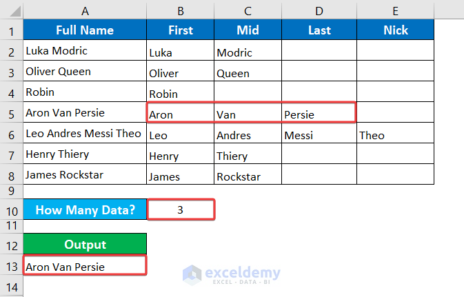
Dear Jae, You have my heartfelt gratitude. I found your queries quite distinctive and innovative. Yes, you can find out Names based on multiple data. Although there is no single functions in VBA that can extract result based on data, you must apply multiple VBA functions such as SPLIT, COUNTA, OFFSET, IF to get the job done.
Step 1: Write the VBA code in the module and hit the Run icon.
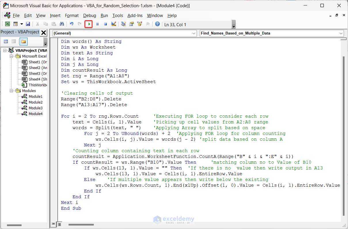
VBA Code
Step 2: Obtain output as follows.
Thanks a ton. Have a good day.
Regards,
MD Tanvir Rahman
Excel and VBA Content Developer
ExcelDemy, Softeko
Hello Nathan, Thanks for your observation. I got your shortcoming. This article focuses on removing links of local storage before opening Excel Spreadsheet files.
However, probably you are likely to remove hyperlinks such as doc links, youtube links, any website links. To remove hyperlinks, you can follow the article: Remove Hyperlinks from Excel Worksheets
I hope now you will be able to fix the issue. For any further shortcomings please let me know. We, team ExcelDemy are ready to assist you.
Thanks a ton. Have a good day.
Regards,
MD Tanvir Rahman
Excel and VBA Content Developer
ExcelDemy, Softeko
Hello! Peter Atallah, Thanks for the Query. It sounds like you’re encountering an issue with the “Find and Replace” feature in Microsoft 365 Apps for Enterprise, where you used to see a message box indicating the number of replacements made, but it’s no longer appearing. Here are a few steps you can try to troubleshoot and resolve this issue:
1. Check Notification Settings: Make sure that notifications are enabled in your Microsoft Office settings. Sometimes, notifications may have been disabled, which could prevent the message box from appearing.
2. Update or Repair Office Installation: Ensure that your Microsoft Office installation is up to date. Sometimes, issues can arise due to outdated software. If updating doesn’t work, you could also try repairing your Office installation. To do this, go to “Control Panel” > “Programs and Features,” select Microsoft Office, and choose “Change.” Then, select “Repair” and follow the prompts.
3. Reset Office Settings: If the issue persists, you can try resetting your Office application settings to their defaults. To do this, open any Office application (e.g., Word), go to “File” > “Options” > “Advanced,” and click the “Reset” button under the “Reset” section. Please note that this will revert all customizations back to their default settings.
Please feel free to let us know the update after trying these approaches.
Thanks a ton. Have a good day.
Regards,
MD Tanvir Rahman
Excel and VBA Content Developer
ExcelDemy, Softeko
Dear Lorenzo Pomini, Thank you so much for your queries. Probably Excel file location is not correct or you forgot to rename a sheet as “January“. However, please follow the mentioned steps. I hope it works.
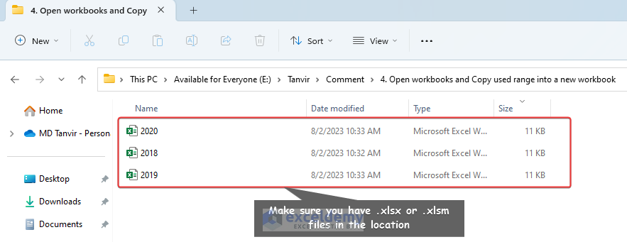
Step 1: Make sure you created 2 or more worksheets in a preferred location.
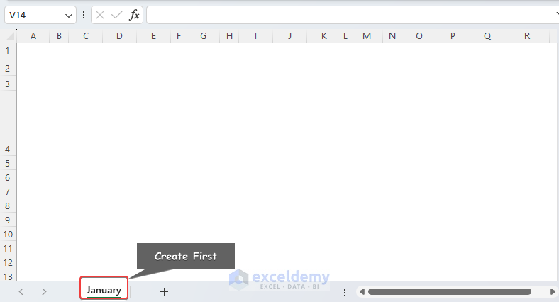
Step 2: Create a worksheet named “January”
Step 3: Insert the following code in the module and hit the Run button.
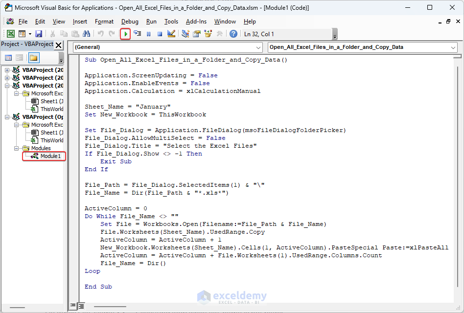
Code Explanation:
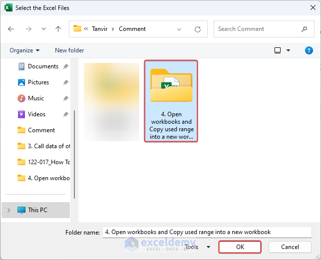
Step 4: Select the folder to where Excel files are located.
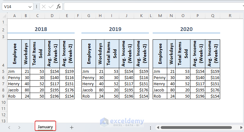
Step 5: Obtain outcome containing data of 2017, 2018, 2019, 2020 in the January worksheet of the active workbook.
I hope these steps will be helpful to you. Please let me know if you face any further shortcomings. Thanks a ton. Have a good day.
Regards,
MD Tanvir Rahman
Excel and VBA Content Developer
Exceldemy, Softeko.
Dear Brittany, Thank you so much for your distinctive query. Here we are setting up a sample dataset of Electronics, Fashion and Snacks category. Using the following formula containing IF function in the D5 cell, you will be able to call the value of cells of the row once it is matched to a cell of same column.
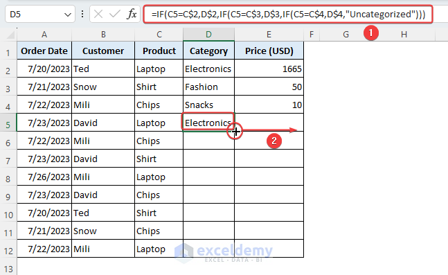
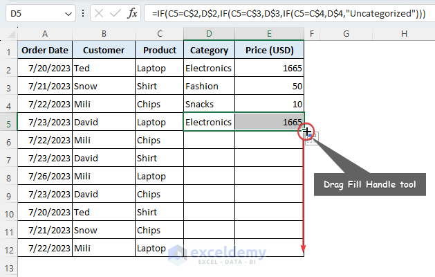
=IF(C5=C$2,D$2,IF(C5=C$3,D$3,IF(C5=C$4,D$4,”Uncategorized”)))
Now drag the Fill Handle tool to fill the cells automatically.
I hope, the solution will be fruitful to you. For any further shortcomings, don’t forget to reach us. Have a good day.
Regards,
MD Tanvir Rahman
Excel and VBA Content Developer
Exceldemy, Softeko
Dear Savvas, You are most welcome. Your encouraging words motivate us a lot. Please stay tuned with Exceldemy for amazing contents.
Regards,
MD Tanvir Rahman
Excel and VBA Content Developer
Exceldemy, Softeko
Hello Asmitha, Thanks for your query. I found it very fascinating. Yes, we can insert a image in the A1 cell and export it to the Outlook in the middle of the email body.
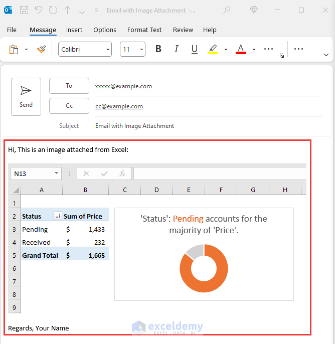
Put the following VBA code in the module and get the output like below image.
Thanks a ton and have a good day.
Regards,
MD Tanvir Rahman
Excel and VBA Content Developer
Exceldemy, Softeko