Applying a Title Cell Style in Excel – 4 Methods

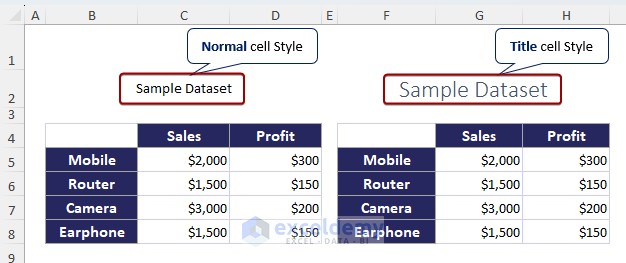
The image below showcases the difference between a normal cell style and a Title cell style in Excel.

Method 1 – Applying a Title Cell Style in Excel

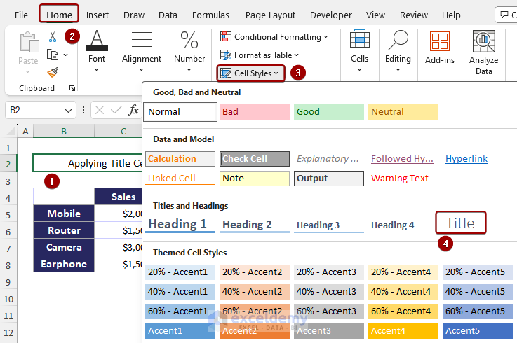
• Select the cell to apply the title cell style.
• Go to the Home tab > Styles > Cell Styles > Title.
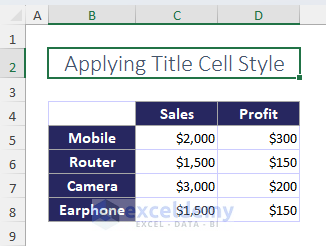
  This is the output.
  

Method 2 – Modifying the Title Cell Style in Excel

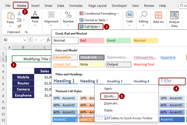
• Go to the Home tab > Cell Styles.
• Right-click a Style and select Modify.
  
• In Style, select Format.
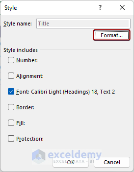  In the Format Cells dialog box, explore 5 options:

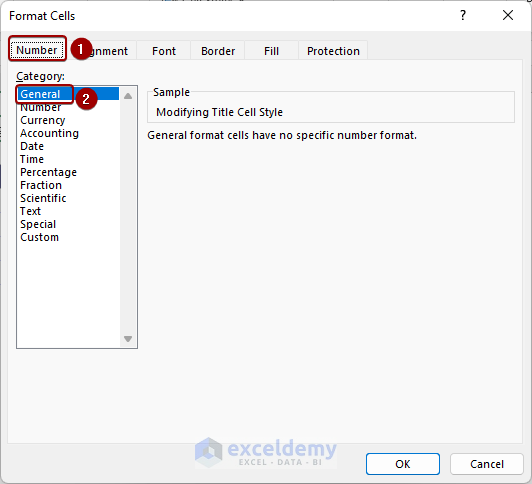
Selecting Number Format

• In the Format Cells dialog box, select Number and choose General.

  

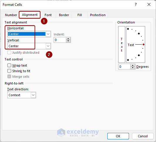
Adjusting Alignment

• Go to the Alignment tab.
• In Horizontal and Vertical, select the how to align texts. Here, Center.
  

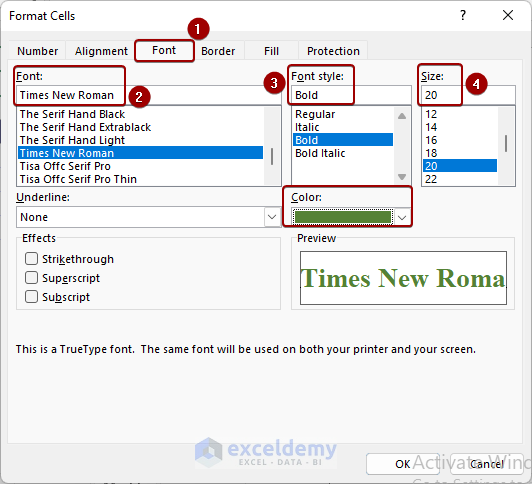
Selecting Font

• Go to the Font tab.
• Select a font. Here, Times New Roman.
• Choose the font style. Here, Bold.
• Select the font size. Here, 20.
• Select the font color. Here, Green, Accent 6, Darker 25%.
  

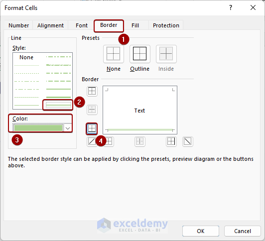
Adding Borders

• Go to Border and select a style. Here, Double Bottom Border.
• Change the border-line color. Here, Green, Accent 6, Lighter 60%.
  

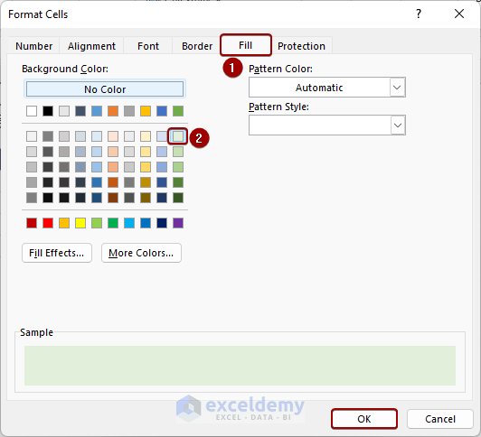
Choosing a Fill Color

• Go to Fill and select a color. Here, Green, Accent 6, Lighter 80%.
• Click OK.
  

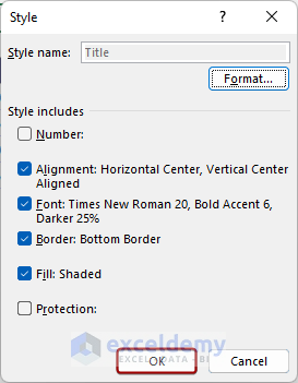
In the Style dialog box, click OK.

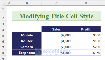
This is the output.

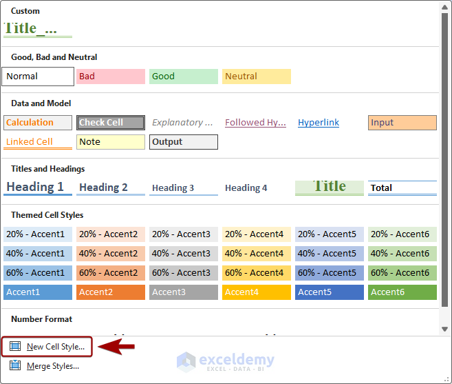
Note: Once you modify the cell style, it can not be reverted to the default cell style. To change it again, go to New Cell Styles and choose Custom.

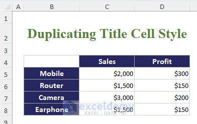
Method 3 – Duplicating the Title Cell Style in Excel

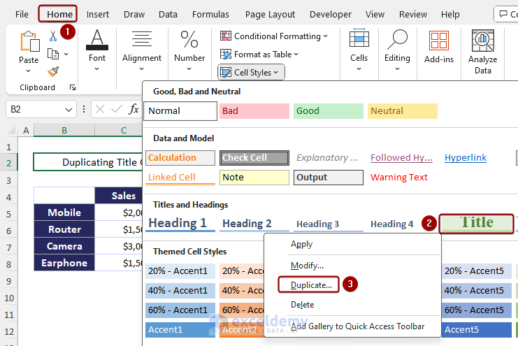
• Go to the Home tab and select Cell Styles.
• Right-Click the Style you want to duplicate and select Duplicate.
  Here, the modified Title command was duplicated.
  
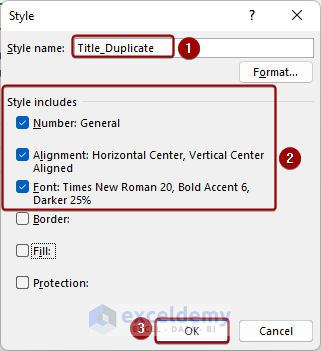
• In the Style dialog box:
  • Enter the Style name. Here, “Title_Duplicate”
  • Check the options to apply: Here, Number, Alignment, and Font.
  • Click OK.

  

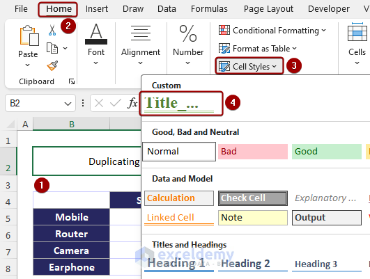
To apply the modified Title cell style in the dataset title:

• Select the cell to apply the title cell style.
• Go to the Home tab > Styles > Cell Styles > Custom  > Title_Duplicate.
  This is the output.

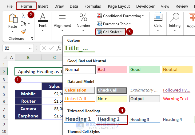
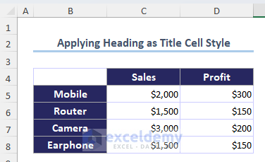
Method 4 – How to Apply the Heading Cell Style as Title in Excel

• Select the data.
• Go to the Home tab > Styles > Cell Styles > Heading 2.
  This is the output.
  

Download Practice Workbook

Frequently Asked Questions

How to remove the Title cell style in Excel?

• Select the data.
• Go to the Home tab > Styles > Cell Styles > Normal.

How to add cell styles in the Quick Access Toolbar in Excel?

• Go to the Home tab > Cell Styles.
• Right-click a style and select Add Gallery to Quick Access Toolbar.

What happens when we delete a cell style in Excel?

If you Right-Click a cell style, and click Delete, you will no longer be able to undo the operation.

<< Go Back to Cell Styles in Excel | Excel Cell Format | Learn Excel