Latest Posts From Maruf Islam
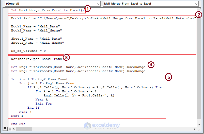
Scenario Often, users have a few customer mailing credentials in an Excel file and need to fetch additional credentials that match existing data in the active ...

The first and foremost way to use Excel is to have information/data. Therefore, users need to organize information in Excel to be able to make interpretable ...

Suppose we have the following dataset containing dates along with other entries, and we want to filter the dataset to only show entries from the last 30 days. ...

Method 1 - Applying Pivot Chart to Group Dates in Excel Inserting a Pivot Chart Step 1: Highlight the range then go to the Insert tab > Click on ...

Suppose we have a dataset of compiled survey data and we want to analyze it. In this article, we'll use multiple formulas and the Power Query method to ...
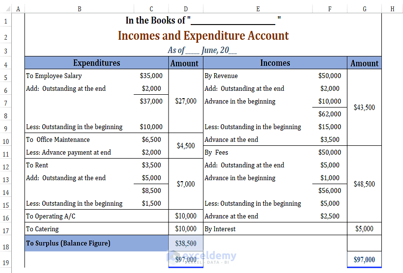
This is a typical Income and Expenditure Account and Balance Sheet. What Is an Income and Expenditure Account? An Income and Expenditure Account is ...

Suppose we have the Sales Amount for the first couple of dates in a month and we want to forecast the sales amount for the rest of the days in the month. ...

The chart below shows basic bond particulars. We will look at how to calculate the bond price. Method 1 – Using Coupon Bond Price Formula Steps: ...
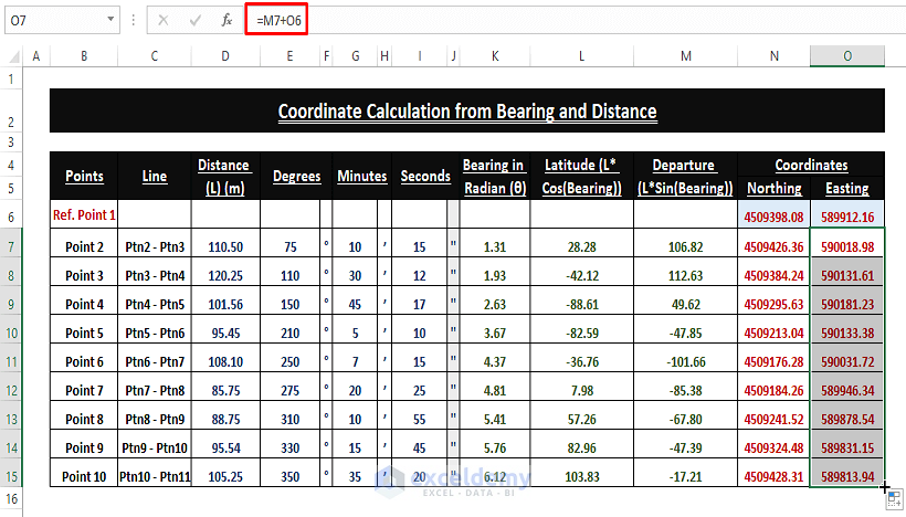
What Are Coordinates (Northing and Easting)? The geographic Cartesian Coordinates of a point on earth are referred to as Easting (the x value), and Northing ...

In Excel, users calculate various Statistics properties to showcase data dispersion. For this reason, users try to calculate the Coefficient of Variance in ...

The dataset showcases the monthly return percentages of Stocks and Bonds. What Is the Mahalanobis Distance? The Mahalanobis Distance (DM) ...

Method 1 - Clicking on 'Enable Editing' to Edit in Protected View When opening an unsafe file (saved in previous versions of Excel or received from external ...
Method 1 - Converting Feet to Meters Using Arithmetic Operations Arithmetic Operations such as Multiplication (i.e., x) or Division (i.e., /) are the basic ...

Watch Video – Create an Autofill Form in Excel What Is an AutoFill Form in Excel? Autofill Form is a data entry or verification tool. ...
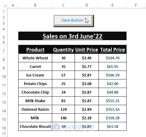
How to Insert a Macro Button and Assign a Macro Before creating a VBA-Enabled Save Button, users must insert a Command Button and assign a Macro to it. ...
- « Previous Page
- 1
- 2
- 3
- 4
- 5
- 6
- …
- 13
- Next Page »
See Our Reviews at


Welcome @Janice
Greetings Jessica,
Use the SUMIFS function to impose multiple criteria like Product Category, Product, and Dates to find out the total sales of products (i.e., Chocolate Chip or Carrot).
For Chocolate Chips
=SUMIFS(G4:G17,E4:E17,J4,F4:F17,J5,B4:B17,">="&J6,B4:B17,"<="&J7)For Carrot
=SUMIFS(G4:G17,E4:E17,M4,F4:F17,M5,B4:B17,">="&M6,B4:B17,"<="&M7)You can also add all the different sales afterward. Hope, this may help you.
Regards
Maruf Islam (Exceldemy Team)
Greetings Ahsan Ahmed,
It’s not clear why you want to use the INDEX-MATCH formula in the first place. However, if I assume you want to use the INDEX-MATCH formula for fetching some matching values, then you want to Add, Subtract, Multiply, or Divide them. You can use the below formula to return the matched values. And afterwards, you can execute any Arithmetic Operations you want.
=IFERROR(INDEX($D4:$D$9,IF(ISNUMBER(MATCH($B$4:$B$9,$F$6,0)),MATCH(ROW($B$4:$B$9),ROW($B$4:$B$9)),""),ROWS($A$1:A1)),"")Hope, the formula may satisfy your cravings.
Regards
Maruf Islam (Exceldemy Team)
Greetings Dr. Linda Vandergriff,
Go through the following methods to get rid of the inconvenience. Make sure the value cells are in the Currency or Accounting Number Format.
1. Manually delete the preceding Apostrophes. Or
2. Use a formula to auto remove the Apostrophes as shown in the image.
=NUMBERVALUE(SUBSTITUTE(B2,"'",""))Feel free to comment if you have further inquiries. We are here to help.
Regards
Maruf Islam (Exceldemy Team)
Greetings Jack Kuehne,
Thank you for your appreciation.
To make static only one (01) calculated cell value or range values, follow the below steps:
1. Unlock all cells within the worksheet using the Format Cells window (CTRL+1 or Home > Click Font Setting Icon to open Format Cells window > Protection > Untick Locked) [Shown in the latter image].
2. Highlight the desired cell or range (you want to keep static no matter what) then Lock them using Step 1 (Tick Locked in the Protection section of Format Cells window).
3. Go to the Preview tab > Tick Select Locked Cells and Select Unlocked Cells > Enter Password > OK > Re Enter Password.
Step 2 and 3 represent Method 1 of this article.
Regards
Maruf Islam (Exceldemy Team)
Greetings Ganesh,
You can find the delivery date using SUM or a simple Arithmetic Formula, as I used in the following picture.
=SUM(B3,7*C3 or D3)or
=B8+7*C8 or D8I hope this solves your seeking. Comment, if you need further assistance.
Regards
Maruf Islam (Exceldemy Team)
Greetings Ashif,
You can manipulate (Hide or Unhide) the Rows of a Protected Worksheet by ticking the Use AutoFilter option under Allow all users of this worksheet to:
[Go to the Review tab > Protect / Unprotect Sheet > Tick Use AutoFilter > Enter Password > Click OK]
I hope this may work in your case. Let me know your thoughts in the comment section.
Regards
Maruf Islam (Exceldemy Team)
Greetings Julian Chen,
Sadly, the HYPERLINK function doesn’t support any attachment links in its arguments. You have to use Other Means to attach files. You can use Method 3 of this article to include an attachment.
Regards,
Md. Maruf Islam (Exceldemy Team)
Greetings Ramin Janani,
This part of the macro takes the 1st brackets as characters to trigger the macro to Color Text or Characters within them. Make sure you encompass the text or characters with brackets. I’ve tested the macro in languages other than English and it works.
Of course, you can change the strCharacter and endCharacter with whatever character (i.e., (),{},[]) you assign to in the macro.
Regards,
Md. Maruf Islam (Exceldemy Team)
Greetings Tom,
You are right. You can calculate the Total Paid or Payable Amount of a loan using PMT*nper or Cumulative Interest + Loan Amount. And the amount will be the same.
Make sure you enter the Start_period (i.e., minimum 1) and End_period (i.e., within the Total Periods (60)) correctly.
Regards,
Md. Maruf Islam (Exceldemy Team)
You are welcomed Jaisinh Chavan. Thanks for your kind words.
Regards
Maruf Islam (Exceldemy Team)
Greetings Mani,
Use the following macro code to copy data (from tables or normal ranges) to the bottom of an existing table (i.e., Table1 or anything).
The macro fetches an input box to select the preferred range to copy and paste afterward. Change the Worksheet Name (i.e., vba) and Table Name (i.e., Table1) as existing table.
Download the Excel file for your better assistance.
https://www.exceldemy.com/wp-content/uploads/2022/09/Macro_to_Copy_Data_to_Bottom.xlsm
Regards
Maruf Islam (Exceldemy Team)
Dear Tijs Tijert,
The used formula shouldn’t react this way. Also, I’m not sure what your data and values are that you used as criteria. Kindly email me your dataset to [email protected]. I’ll try my best to come up with a solution to your problem.
Regards
Maruf Islam
Greetings Joseph Clovis,
The AND and FILTER functions do take cell references to filter and fetch entries that fall under the condition
(Date>= T0DAY()-30 <TODAY())respectively. However, sadly, the Excel Filter feature doesn’t support selecting dates from ranges or entries. All the Filter execution does is that it hides rows, which may lead to inconveniences sometimes. Till now, there has been no alternative to selecting dates from the Filter dialog box options. But you can try Conditional Formatting or VLOOKUP function for highlighting and fetching data. And in those cases, you can use cell references from your dataset.1. Conditional Formatting: Highlight Cells or Range > Go to Home > Conditional Formatting > New Rule > Select a Rule Type and Format > OK.
=AND($B5>=(TODAY()-30),$B5<TODAY())2. VLOOKUP Function: Use TODAY()-30 in any cell, then use the VLOOKUP formula to fetch different entries. In that way, the dataset range remains intact.
=TODAY()-30=VLOOKUP(F5,$B$5:$D$16,2,0)=VLOOKUP(F5,$B$5:$D$16,3,0)Hope, these ways help you to compensate the Excel Filter caveats. Feel free to comment if the solution doesn’t satisfy your seeking. Our Exceldemy Team is always there to help.
Greetings Indra,
Thanks for your appreciation.
The probable causes behind the freezing of Visual window or Excel are:
1. VBA Macros use device’s single core to run or execute macros.
2. Large data normally take several minutes to complete any macro-driven outcomes. Therefore, sudden freezing of visual window or Excel is common among users.
You can use the already used macro (in the article), if it works fine after couple of minutes of freezing or unresponsiveness. Otherwise, email us your Data to get custom macro that may solve the issue (As we don’t have such huge data to test our code with). Also, you can go through:
1. Divide your data into worksheets then execute the macro individually. Then merge the worksheets into one.
2. Use other means such as formulas to accomplish the desired outcome.
Hope, it helps you. Comment if further issues arise.
Hi Taylor,
# The macro contains conditions against the email sending within a Week prior to the Deadline/Due Date using the following line
# So, the email will get sent within- 1 day <= Deadline/Due Date <= 7 day or 1 week range prior to the Deadline/Due Date.
Hope, you find your answer, let us know if further explanation is needed. Our dedicated Softeko Team is always there to help.
Greetings Sepehr,
Thank you for your appreciation.
# The answer to your question is “Yes“—it is possible to have the list of products in different columns.
# Just use the TRANSPOSE function preceding the UNIQUE+XLOOKUP formula. Of course, you have to have Excel 365 to use the XLOOKUP function.
=TRANSPOSE(UNIQUE(XLOOKUP(B5,B7:D7,B8:D14),,TRUE))Hlw Melissa,
I’m assuming you need to Data Validate multiple selection G7 to H15 (adjacent columns) or whatever the cell is.
# Modify the 1st IF Condition as ” If Not Intersect(Target, Range(“G7:H15″)) Is Nothing Then ” or Change the ” Range(“G7:H15″) ” portion with Capital Letters. Of course don’t forget to apply Data Validation to those cells first.
Hope this works. Otherwise, comment with detailed cell references.
Regards
Maruf
Hlw Kim, Sorry for being late.
# Excel Pivot Table normally considers multiple items within a cell as “1”. Therefore, multiple selection within a cell doesn’t have any effect on count. However, conditional counting may have different issue.
Hlw Reena Pujari. Sorry for late reply.
To apply macro to all cells in the same column, follow:
1. Apply “Data Validation” to all the cell of a column (Highlight Entire Column > go to “Data” > apply “Data Validation”)
2. Replace ” If Target.Address = “$D$4″ Then ” line within the macro (with repetition or without repetition) with ” If Not Intersect(Target, Range(“D:D”)) Is Nothing Then “.
Hlw Avery, Sorry for late reply.
To duplicate this for more than 1 multiple select list option:
# Replace ” If Target.Address = “$D$4″ Then ” line within the macro (with repetition or without repetition) with ” If Not Intersect(Target, Range(“D4:D5”)) Is Nothing Then “.
Note: You can have multiple Source ranges assigned for “Target.Address” s using Data Validation.
Thanks for your appreciation @Ed
You can exclude or ignore the blanks using 2 simple tricks.
1. Use an additional formula in conditional formatting. Go to conditional formatting > New Rule option > select Format Only Cell that contains rule type > Select Blanks from edit rule description > Keep Cell format as no cell format. Click OK.
2. Go to Conditional formatting > New Rule option> Select Use a formula to determine which cell to format rule type > type “=ISBLANK(Cell Reference)=TRUE” in the Edit the Rule description box > Keep Cell format as no cell format. Click OK.
Hope these tricks work for you.