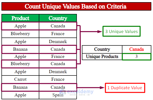
Imagine we have an Excel file containing data about various fruits exported by a businessman to different European countries. The dataset includes two columns: Product Name and Country of Export. Our goal is to count the unique types of fruits based on specific criteria in the other column. In the example below, we’ve determined and counted the number of distinct fruit types sent to Canada:
Method 1 – Using UNIQUE, LEN, and FILTER Functions (for Microsoft Office 365 users)
- Background:
- If you’re using Microsoft Office 365, the easiest way to achieve this is by utilizing the UNIQUE function exclusively in Excel 365.
- We’ll count unique values based on criteria in another column.
- Steps:
- Open your Excel workbook and navigate to the sheet where you want to perform this operation.
- Let’s assume you have data in columns B (Product) and C (Country).
- We want to count unique product types exported to Canada.
- Formula:
- In cell F9, enter the following formula:
=SUM(--(LEN(UNIQUE(FILTER(B5:B14,C5:C14=F8,"")))>0))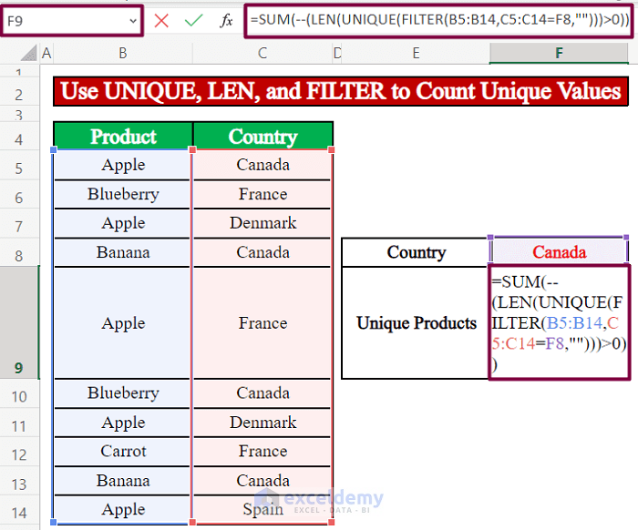
- Formula Breakdown:
- The FILTER function will return cells from the Product column where the corresponding cell values in the Country column are Canada (F8).
- The UNIQUE function will extract unique values from the filtered cell values.
- The LEN function checks if the length of each unique item extracted by the UNIQUE function is greater than zero (0). It returns TRUE if the length is greater than zero, otherwise FALSE.
- We use double minus signs (– –) to transform TRUE and FALSE values to 1 and 0, respectively.
- We sum up the values in this list to get the total count of unique product types.
- Result:
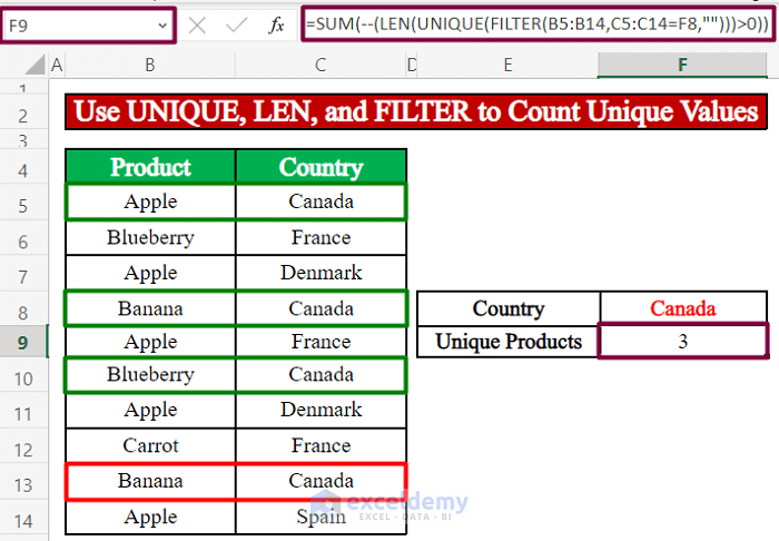
- After pressing ENTER, you’ll obtain the total count of unique fruit types exported to Canada.
- For example, if the businessman exported fruits to Canada four times, but Banana was exported twice, the formula will count cell B13 as a duplicate. Therefore, it returns 3 as the total count of unique fruit types exported to Canada.
- Additional Criteria:
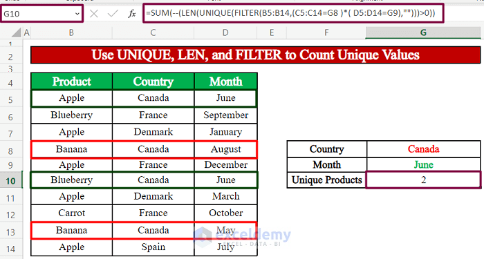
- You can include multiple criteria from different columns. For instance, if you’ve added a Month column indicating when a specific product is exported to a country, you can use the Month column as a second criterion along with the Country column to count unique fruit types exported to Canada in June.
- Enter the following formula in cell G10.
=SUM(--(LEN(UNIQUE(FILTER(B5:B14,(C5:C14=G8)*(D5:D14=G9),"")))>0))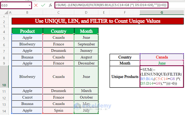
- Now, let’s break down this formula:
- FILTER Function:
- The FILTER function will return cells from the Product column (B5:B14) where both of the following conditions are met:
- The corresponding cell values in the Country column (C5:C14) are Canada (G8).
- The corresponding cell values in the Month column (D5:D14) are June (G9).
- The FILTER function will return cells from the Product column (B5:B14) where both of the following conditions are met:
- UNIQUE Function:
- The UNIQUE function will extract unique values from the filtered cell values obtained from the previous step.
- LEN Function:
- The LEN function checks if the length of each unique item extracted by the UNIQUE function is greater than zero (0). It returns TRUE if the length is greater than zero, otherwise FALSE.
- Double Minus Signs (- -):
- We use double minus signs to transform TRUE and FALSE values to 1 and 0, respectively.
- SUM Function:
- Finally, we sum up the values in this list to get the total count of unique product types exported to Canada in June.
Result:
- After pressing ENTER, the cell will return 2 as the total count of unique types of fruits exported to Canada in June.
- This calculation excludes cells B8 and B13, considering that Banana was exported twice during that month.
- FILTER Function:
Method 2: Using UNIQUE, ROWS, and FILTER Functions (for Microsoft Office 365 users)
- Background:
- In this method, we’ll merge the UNIQUE, ROWS, and FILTER functions to achieve our goal.
- We want to count unique product types exported to Canada based on specific criteria.
- Formula:
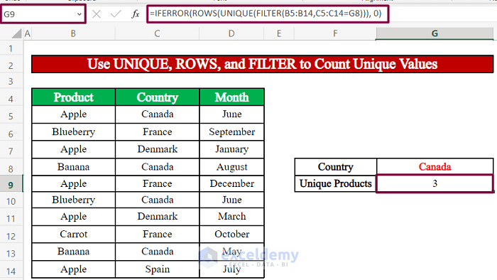
- In cell G9, enter the following formula:
=IFERROR(ROWS(UNIQUE(FILTER(B5:B14,C5:C14=G8))),0)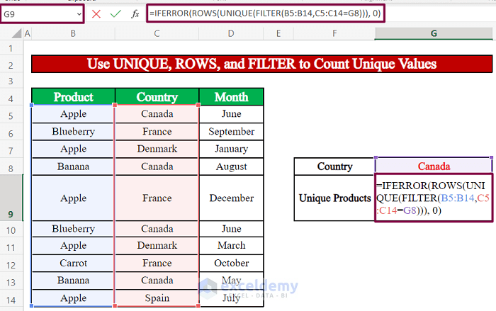
- Formula Breakdown:
- The FILTER function will return cells from the Product column (B5:B14) where the corresponding cell values in the Country column (C5:C14) are Canada (G8).
- The UNIQUE function will extract unique values from the filtered cell values.
- The ROWS function counts the number of rows (unique items) returned by the UNIQUE function.
- The IFERROR function ensures that if there are no unique values, it returns 0 instead of an error.
- Result:
- After pressing ENTER, the cell will display the total count of unique fruit types exported to Canada.
- For example, if the businessman exported fruits to Canada four times, but Banana was exported twice, the formula will exclude cells B8 and B13. Therefore, it returns 2 as the total count of unique fruit types exported to Canada.
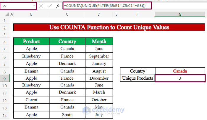
Method 3: Using the COUNTA Function (for Microsoft Office 365 users)
- Background:
- In this method, we’ll utilize the COUNTA function to achieve our goal.
- We want to count unique product types exported to Canada based on specific criteria.
- Formula:
- In cell G9, enter the following formula:
=COUNTA(UNIQUE(FILTER(B5:B14,C5:C14=G8)))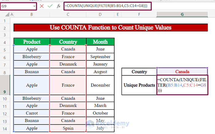
- Formula Breakdown:
- The FILTER function will return cells from the Product column (B5:B14) where the corresponding cell values in the Country column (C5:C14) are Canada (G8).
- The UNIQUE function will extract unique values from the filtered cell values.
- The COUNTA function will count all the unique cell values returned by the UNIQUE function.
- Result:
- After pressing ENTER, the cell will display the total count of unique fruit types exported to Canada.
- For example, if the businessman exported fruits to Canada four times, but Banana was exported twice, the formula will exclude cells B8 and B13. Therefore, it returns the correct count of unique fruit types exported to Canada.
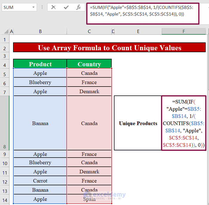
Method 4: Using an Array Formula
- Background:
- If you’re familiar with array formulas, you can use them to achieve this task.
- We want to count the unique countries where apples were exported by the businessman.
- Formula:
- In cell G9, enter the following array formula:
=SUM(IF("Apple"B5:B14,1/(COUNTIFS(B5:B14,"Apple",$C$5:$C$14,$C$5:$C$14)),0))-
-
- Note: This is an array formula. To insert it in a cell, press CTRL+SHIFT+ENTER together. The formula will be enclosed in curly braces.
-
- Formula Breakdown:
- The COUNTIFS function counts the number of cells within a range that meet the given condition (in this case, where the product is “Apple”).
- The IF function allows you to make logical comparisons between a value and your expected condition.
- The SUM function then adds up all the values from this list to return the total count of unique values.
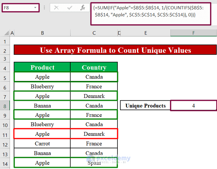
- Result:
- After pressing ENTER, the cell will display the total count of unique countries where apples were exported.
- For example, if the businessman exported apples to four unique countries, but Banana was exported twice, the formula will exclude the duplicate entries. Therefore, it returns 4 as the total count of unique countries.
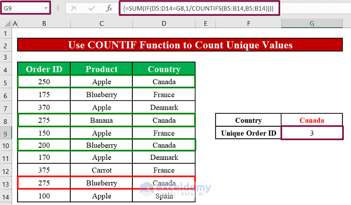
- Additional Example (Using COUNTIF):
- You can also use another array formula with the COUNTIF function to count unique Order IDs of orders sent to Canada.
- Follow the same steps, and in cell G9, enter the appropriate formula for counting unique Order IDs.
=SUM(IF(D5:D14=G8,1/COUNTIFS(B5:B14,B5:B14)))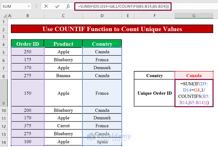
- When you press ENTER, you’ll receive the unique Order IDs for the orders sent by the businessman to Canada. Out of the 4 orders sent, 3 have distinct order IDs, while the remaining one shares an order ID with one of those 3 unique IDs. As a result, the formula returns a count of 3 unique order IDs for the orders destined for Canada.
Quick Notes
- Array Formulas (Methods 4 and 5): When using formulas from methods 4 and 5, remember that they are array formulas. To insert them into a cell, press CTRL+SHIFT+ENTER together. This action will enclose the entire formula in curly braces.
- UNIQUE Function (Excel 365 Only): The UNIQUE function is currently exclusive to Excel 365. If you’re not using Excel 365 on your PC, this function won’t work in your worksheet.
Download Practice Workbook
You can download the practice workbook from here:
<< Go Back to Count | Unique Values | Learn Excel
Get FREE Advanced Excel Exercises with Solutions!
