Method 1 – Finding Duplicate Values in Excel with INDEX, MATCH, IF, and COUNTIF
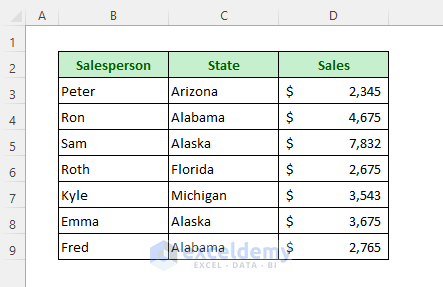
We have input some salespersons’ states and sales in the dataset. Now we’ll find duplicate values. If no duplicate is found, then the formula will show “Original” and if there is any duplicate then it will show “Duplicate”.
Steps:
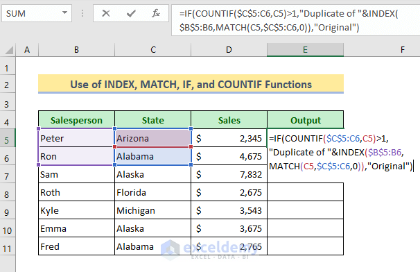
- Select Cell E5
- Copy the following formula into it:
=IF(COUNTIF($C$5:C6,C5)>1,"Duplicate of "&INDEX($B$5:B6,MATCH(C5,$C$5:C6,0)),"Original")- Hit Enter to get the output.
- Double-click the Fill Handle icon (bottom-right corner of the cell) to copy the formula for the other cells.
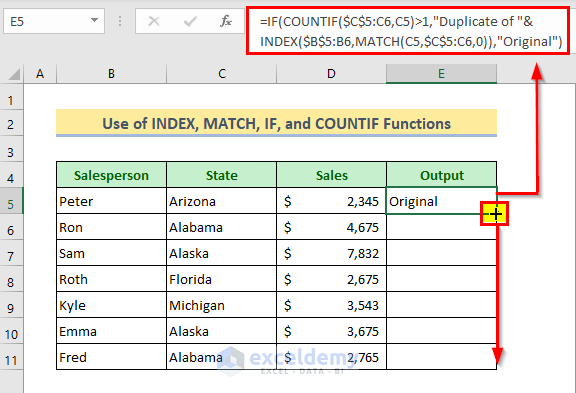
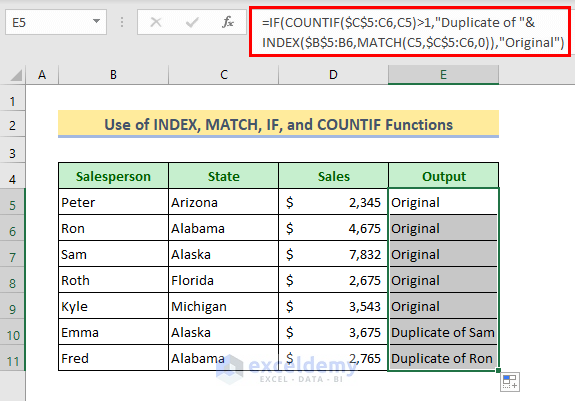
- You will see whether duplicates exist in the dataset.
💡 Formula Breakdown:
➥ MATCH(C5,$C$5:C6,0)
The MATCH function finds the first occurrence of a value in a stack of values and returns the relative row number where the value is found. So it returns as-
{1}
➥ INDEX($B$5:B6,MATCH(C5,$C$5:C6,0))
The INDEX formula returns a value from a specified row of a specified stack of cells. Like, INDEX(B1:B10,5) would return the 5th value in the range B1:B10. From our array it will return as-
{Peter}
➥ COUNTIF($C$5:C6,C5)>1
The COUNTIF function will look at all the states so far and counts up how many times the current value has occurred. If Excel sees the current value for the first time, the formula returns 1. And as 1 is not greater than 1, so it will show-
{FALSE}
➥ IF(COUNTIF($C$5:C6,C5)>1,”Duplicate of “&INDEX($B$5:B6,MATCH(C5,$C$5:C6,0)),”Original”)
Finally, the IF function will show “Original” for FALSE and Duplicates for TRUE. So it returns-
{Original}
Method 2 – Joining Excel INDEX, ROW, and SMALL Functions for Duplicate Values
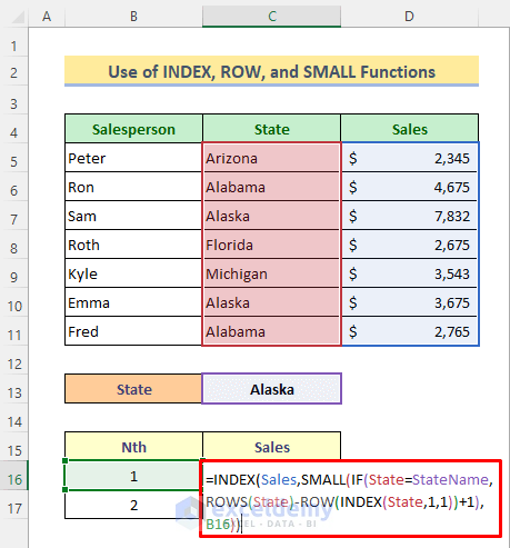
Let’s find the duplicate values of a single given cell (in this case, a state) and list the sales amounts for it.
Steps:
- In Cell C16, insert this formula:
=INDEX(Sales,SMALL(IF(State=StateName,ROW(State)-ROW(INDEX(State,1,1))+1),B16))Note:
We have defined array and reference names that will be used in the formula for easier overview:
Sales= D5:D11
State= C5:C11
StateName= C13
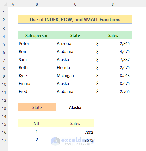
- Hit Enter.
- Copy the formula down with the Fill Handle tool.
⏬ Formula Breakdown:
➥ INDEX(State,1,1)
The INDEX function will return the value according to its relative row number 1 and column number 1. That is-
“Arizona”
➥ ROW(INDEX(State,1,1))
Then the ROW function will find its original row number-
{5}
➥ ROW(State)-ROW(INDEX(State,1,1))+1
As the upcoming INDEX function works for row number of a particular array, not for Excel row number, we have to give the INDEX function the row numbers by applying this formula. The output is-
{1;2;3;4;5;6;7}
➥ IF(State=StateName,ROW(State)-ROW(INDEX(State,1,1))+1)
Then the IF function will do the logic test for the value “Alaska”. If found then it will show the position number whether it will show FALSE and that will return as-
{FALSE;FALSE;3;FALSE;FALSE;6;FALSE}
➥ SMALL(IF(State=StateName,ROW(State)-ROW(INDEX(State,1,1))+1),B16)
The SMALL function will show the lowest number among them which is-
{3}
➥ INDEX(Sales,SMALL(IF(State=StateName,ROW(State)-ROW(INDEX(State,1,1))+1),B16))
The INDEX function will extract the value according to the output of the SMALL function, that returns-
{7832}
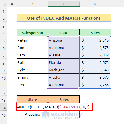
Method 3 – Extracting Values Based on Duplicates in Two Columns with INDEX-MATCH
Let’s extract the sales values for the states of Florida and Alabama.
Steps:
- Copy the formula given below in Cell C14:
=INDEX(C5:D11, MATCH($B14,C5:C11,0),2)- Hit Enter to get the result.
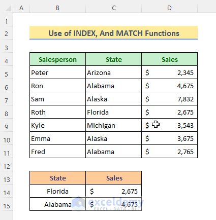
- Use the Fill Handle tool to copy the formula to the cell below.
⏬ Formula Breakdown:
➥ MATCH($B14,C5:C11,0)
The MATCH function will find the relative position for the state “Florida” from the state column, which returns-
{4}
➥ INDEX(C5:D11, MATCH($B14,C5:C11,0),2)
Finally, the INDEX function will extract the sales value according to row number 4 and column number 2 relative to the array C5:D11. That will return as-
{2675}
Download Practice Workbook
You can download the Excel workbook that we’ve used to prepare this article.
<< Go Back to INDEX MATCH | Formula List | Learn Excel
Get FREE Advanced Excel Exercises with Solutions!

Hi, nice tutorial, but I am a begginer.
I would like to make excel table for ordinary tennis league, but if 2 teams are equal with same points than it should take into account their mutual match, so who won the match is higher ranking. So, I have 12 teams, namely:
Team 1
Team2
Team3
Team4
Team5
Team6
Team7
Team8
Team9
Team10
Team11
After entering the results for each round, let Excel itself sort the Teams in the following order:
a) Team with most points is highest ranking.
b) If 2 teams with the same nr. of points, the head-to-head is then watched and whoever won is higher ranking. If the teams have not yet played each other or have result for draw, then skip to c).
c) If the teams are still the same, then they are judged by goal difference – higher difference is higher ranking.
d) If the teams are still the same, then see who received fewer goals – who received less goals is higher ranking..
e If the teams are still the same, then see who scored more goals – who scored more goals is higher ranking.
f) If the teams are still the same, then they occupy the same ranking place.
Here is link for demo file:
https://docs.google.com/spreadsheets/d/1MvQz0USGOsceyaHEFGpgTNRPL9hxbGGR/edit?rtpof=true&sd=true
If you have any solution / formula, pls let me know
Regards
Hello Mat, thanks for your feedback. The problem you mentioned will need a complex formula. You will have to apply a formula like this:
=IF(SUM(–(MAX(AC2:AC12)=AC2:AC12))=1,INDEX(T2:AC12,MATCH(MAX(AC2:AC12),AC2:AC12,0),1)).
Hello Mithun,
I’m trying to do something similar but am having a difficult time applying. I hope you can help with the following:
I have a sheet with thousands of rows representing individual books. However, multiple individual items (books) can be a part of a single title. Each item has usage numbers. Also, each row has unique key for the catalog (catalog ID) and a unique key for the item (item barcode).
I’m looking for two formulas. One to count the number of items per title (according to catalog id). And another to sum the total item usage of all items on the same title.
I’ve included a sample sheet to help illustrate:
https://docs.google.com/spreadsheets/d/1IZOKV46uFo52R0w9dMvHoK1Luj-VHZpt/edit?usp=sharing&ouid=118360611201546687127&rtpof=true&sd=true
I’m looking for formulas to return the values seen in columns E and F.
Any help will be greatly appreciated!
Hello Mithun,
You have created some great instructions! So I’m reaching out for assistance for, possibly, the second time.
If you have already seen a comment by me today, I apologize for the duplication. I posted something earlier but there was no indication that a comment had been submitted. Given your expertise, I thought it would be worth trying again!
I have a sheet with thousands of rows, each row with data about a single item (book). Each item has information such as number of uses and the catalog title to which that item is associated. The same catalog title can be associated with multiple items (think of a multi-volume set of books, all with the same title). Each item has a unique key (item barcode) and each title has a unique key (catalog id).
I am looking for two formulas to help examine usage. One formula will simply count the number of items associated with each title (according to catalog id), returning that value to each row. The other formula will sum the total number of uses of each item associated with that same title, returning that value to each row.
I’ve included an example sheet to demonstrate:
https://docs.google.com/spreadsheets/d/1IZOKV46uFo52R0w9dMvHoK1Luj-VHZpt/edit?usp=sharing&ouid=118360611201546687127&rtpof=true&sd=true
On the example sheet, I’m looking for formulas to return the values in columns E and F.
Any help will be most appreciated!
Hi MICHAEL,
Thanks for your feedback.
To count the number of items associated with each title (according to to catalog id), use this formula: =COUNTIF($B$2:$B$27,B2)
And to sum the total number of uses of each item associated with that same title, use this formula: =SUMIF($B$2:$B$27,B2,$D$2:$D$27)
the duplicates in the first example seem wrong. The dups are being identified by states and Michigan is marked as a duplicate, but it is not. Alabama is a duplicate, but is tagged as original.
Hi TOM,
Thank you so much for letting us know. The formula has been edited. Thanks for your concern. Stay connected!
Regards,
Rafi
Author: ExcelDemy Team
i am preparing a result sheet
in which there are 4 different worksheets in excel with each semester marks of all students
in 5th worksheet i am calling the top 10 scorers from each semester
everything was fine, i used formula
=INDEX(‘Semester 2’!C10:C46,MATCH(LARGE(‘Semester 2′!L10:L46,4),’Semester 2’!L10:L46,0))
but issue arose when i saw 4 and 5 has both same names
however the names should be different
because 2 different students scored same marks
so this formula is calling 1st from both same scorers
how to handle this
else 1 to 3 and 6 to 10 are fine
since their scores were unique
so guide me how can i deal with students who secured same marks using such formula
Hello Naureen,
Thank you for sharing your problem. I am replying on behalf of ExcelDemy. Assuming the student names are in Column A and the scores are in Column B, insert this formula to get the top 10 scorers with duplicate values.
=INDEX(SORT(A2:B16,2,-1),SEQUENCE(10),1)If you want to get the names in another sheet, then just add the worksheet names in the formula (as shown below) and you will get your required output.
=INDEX(SORT(‘Semester 2’!A2:B16,2,-1),SEQUENCE(10),1)I hope this solution will help you. Otherwise, feel free to share your workbook with [email protected] and we will look into this deeply.
Regards,
Guria
ExcelDemy
This is great content and it looks like exactly what I need. I’m running into issues with getting it setup though. My data looks like the following. I need to search Column A for all the times that Item 1 appears and report back the results of the content in column B and C. Any help would be appreciated.
Column A
Item 1
Item 1
Item 1
Item 2
Item 3
Column B
Thing 5
Thing 6
Thing 7
Thing 5
Thing 5
Column C
Display 1
Display 2
Display 3
Display 2
Display 3
Hello Jon,
Thank you for sharing your query. I have gone through your shared dataset but the values and their required output seem quite unclear in your question. Still, I have tried to solve it. You will find the solution in the Excel file below.
https://www.exceldemy.com/wp-content/uploads/2023/04/Index-match-duplicate-values.xlsx
Please go through it and let us know if it is the solution that you are looking for. Otherwise, feel free to share your Excel file with [email protected] and we will look into this deeply.
Thank you.
Regards,
Sanjida Mehrun Guria
Excel VBA & Content Developer
ExcelDemy
Thank you very much!
It helps. 🙂
Hello Joedel,
You are most welcome.
Regards
ExcelDemy