Create a Unique List in Excel Based on Criteria (9 Methods)

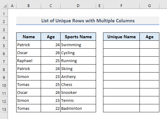
Method 1 – Create a List of Unique Rows with Multiple Column Criteria

In the following dataset, we have a list of players, their ages, and what sport they participate in. The table on the right is the output table where we’ll extract data based on the unique values only. For example, we want to know the names of the unique participants only along with their ages.

The generic formula of the UNIQUE function is:

=UNIQUE(array, [by_col], [exactly_once])

The UNIQUE function is only available in Microsoft 365.

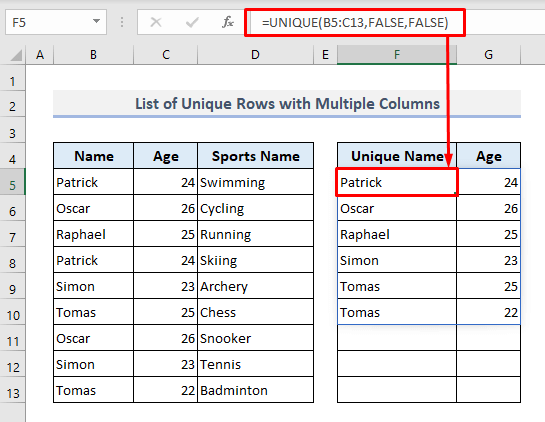
• Insert the following function in cell F5:

• Press Enter, and the function returns a spill range into a column.

Read More: How to Generate List Based on Criteria in Excel

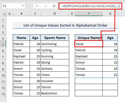
Method 2 – Get a List of Unique Values Sorted in Alphabetical Order

• In the output cell E5, the required formula will be:

• After pressing Enter, the function will return the array sorted in alphabetical order by A to Z.

Read More: How to Make Alphabetical List in Excel

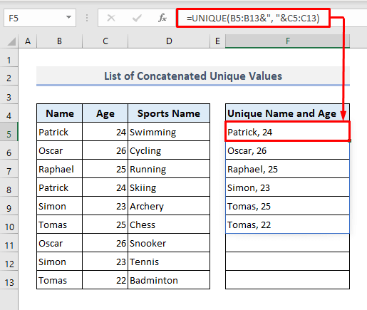
Method 3 – Make a List of Unique Values Concatenated into One Cell

Let’s extract the values for each player into a single cell.

• The required formula in the output Cell F5 will be:

• The formula will return an array of unique rows in a single column.

Read More: How to Make a Comma Separated List in Excel

Method 4 – Create a List of Unique Values with Criteria (UNIQUE-FILTER Formula)

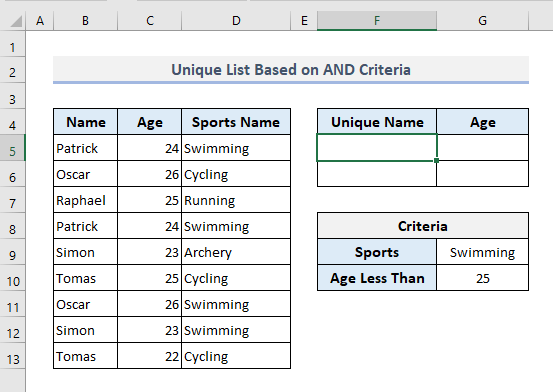
Case 1 – Identify Unique Values Based on Multiple AND Criteria in Excel

We’ll add a few criteria and extract unique data based on those conditions. For example, we want to know the unique names of the participants who have participated in swimming only and are below 25 years old.

• The formula for the output cell F5 will be:

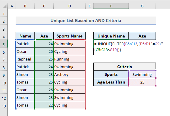
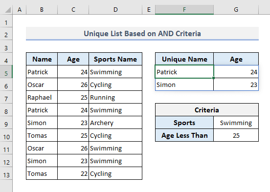
• After pressing Enter, the formula will return a spill array with the unique names and the corresponding ages based on the selected criteria.

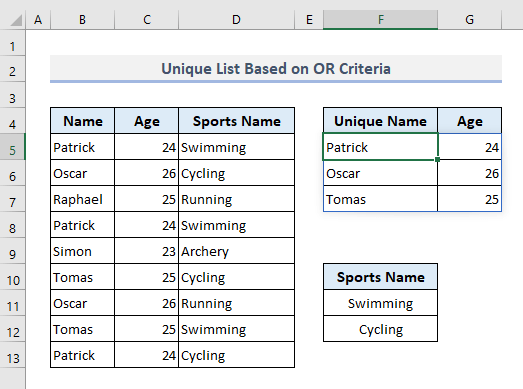
Case 2 – Search Unique Values Based on Multiple OR Criteria

Let’s search for unique participants who took part in swimming, cycling, or both. These sports are listed in a separate column.

• The required formula in cell F5 will be now:

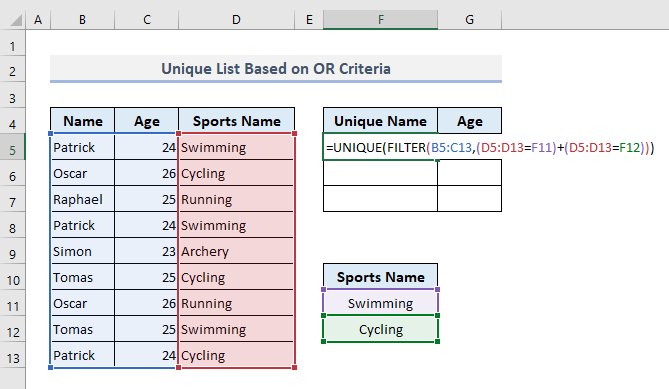
• Press Enter, and you’ll get the extracted unique data in a spill range.

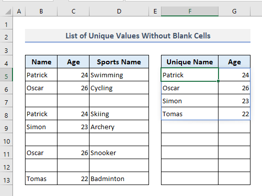
Case 3 – Get a List of Unique Values Ignoring Blank Cells

Let’s input a few blank values into the dataset. We’ll now force the formula to ignore those.

• The required formula in the output cell F5 will be:

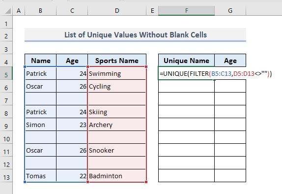
• Press Enter to apply the formula, and it will return an array of non-blank unique values in a spill range.

Read More: How to Make a To Do List in Excel

Method 5 – Find a List of Unique Values in Specified Columns in Excel

From our data table, we’re going to extract the names of the unique participants and show the outputs from the Name (Column B) and Sports Name (Column D) columns only.

• The required formula in Cell F5 will be:

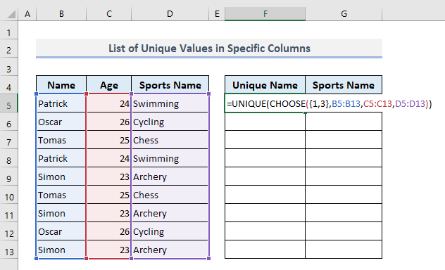
• Apply the formula to get the results.

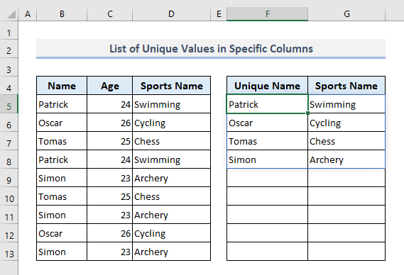
Inside the CHOOSE function, the index numbers are 1 and 3 which implies that the 1st and 3rd arrays of cells have to be selected from the list of values. The UNIQUE function then considers the specified columns only and returns the unique data from those columns in an array.

Read More: How to Make a Numbered List in Excel

Method 6 – Use the IFERROR Function While Creating a Unique List

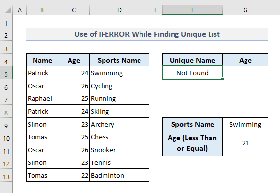
Let’s say we’re checking for the names of unique participants who are under 21. Since there aren’t any, the formula should return a #N/A error. Let’s instead display a customized message “Not Found”.

• Insert the following formula in Cell F5:

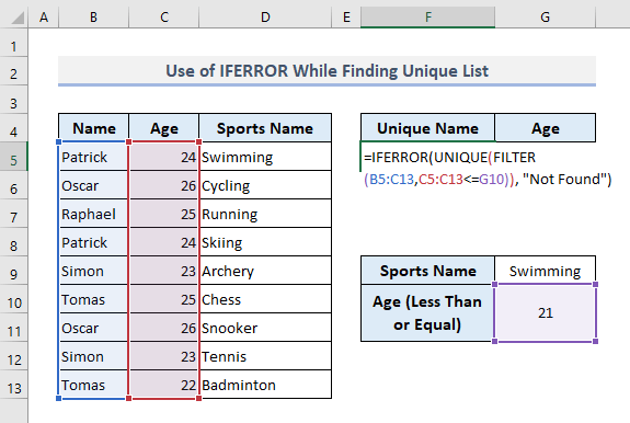
• The formula will return the specified message as shown in the following screenshot if it doesn’t find any results.

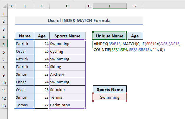
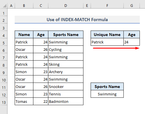
Method 7 – Extract a Unique List Based on Criteria (INDEX-MATCH Formula)

You can apply this method in other versions of Excel.

Steps:

• Select the output Cell F5 and insert the following formula:

• Press Enter.

• Use the Fill Handle to drag the cell to the right.
• This will fetch the age of the participant.

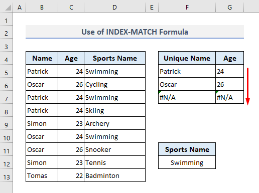
• From Cell G5, fill down the column until a #N/A value appears.

How Does the Formula Work?

• COUNTIF($F$4:$F4, $B$5:$B$13): The COUNTIF function here has been used to store and count all the cells available in the range of B5:B13. And the function returns as:

{0;0;0;0;0;0;0;0;0}

• IF($F$12=$D$5:$D$13, COUNTIF($F$4:$F4, $B$5:$B$13), “”): The IF function searches for the given criteria in the cells and returns as:

{0;””;0;””;””;0;””;””;””}

• The MATCH function returns the row number of the cell found in the previous step.
• Finally, the INDEX function extracts data based on those row numbers.

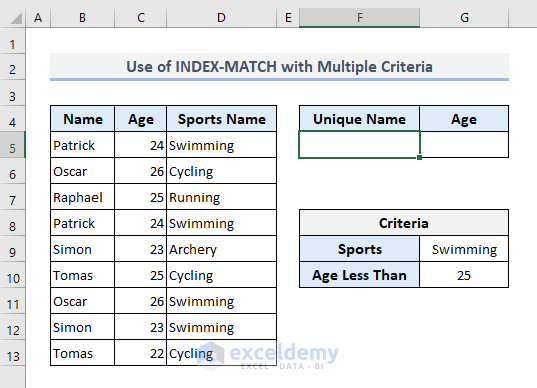
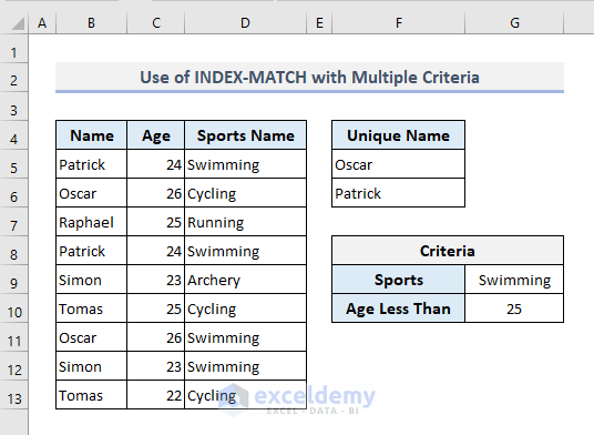
Method 8 – Prepare a Unique List in Excel Based on Multiple Criteria

Let’s fetch the unique names of the participants who have participated in swimming and are younger than 25.

• The required formula in the output cell F5 will be:

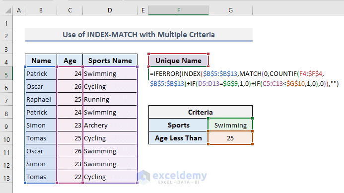
• Press Enter and AutoFill down the column.

In this formula, we have assigned the criteria with two IF functions and the COUNTIF function will consider those criteria while extracting the array of output cells. As described in the previous method, the INDEX-MATCH formula will return the output based on that array. And the IFERROR function here has been used to return a customized message if any error is found.

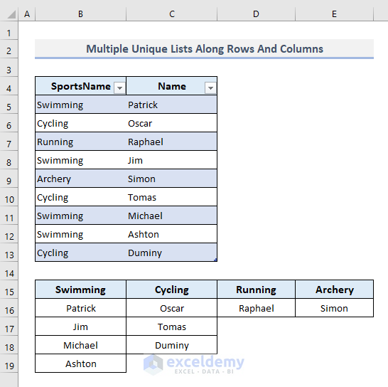
Method 9 – Make Multiple Unique Lists Along Rows and Columns with Criteria

We’ve modified the dataset slightly. The table at the bottom will show the unique names of the participants per sport.

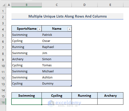
• We’ve named the range of cells (B5:C13) as Sports.
• The columns have headers with the names- SportsName and Name. You must keep in mind that the headers in the table cannot occupy any space.
• Insert the following formula in B16:

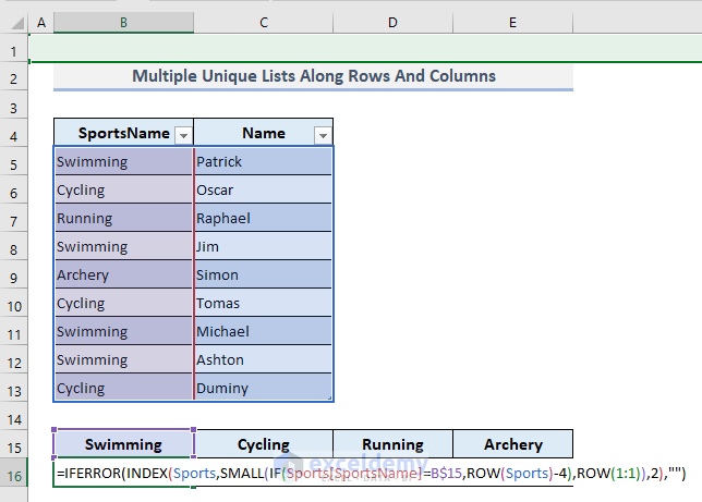
• Press Enter.
• Use the Fill Handle to fill down the column until a blank cell appears.

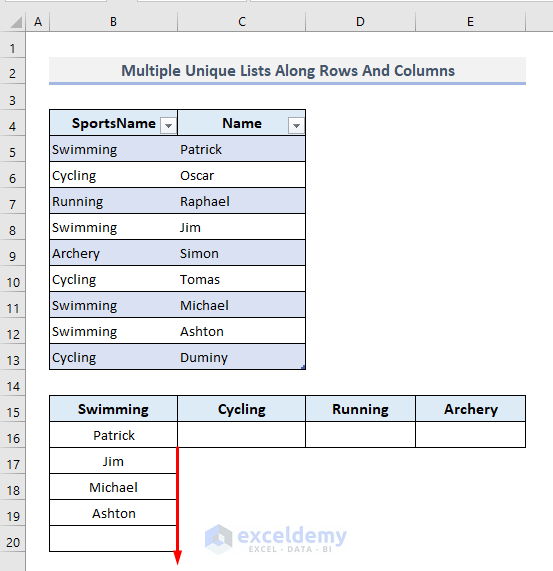
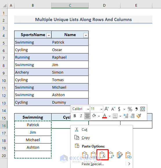
• Copy the range of cells (B16:B20) in the first column.
• In Cell C16, paste the values with the Formulas (F) option.
• AutoFill down until you get a blank cell.

• Repeat for cells D16 and E16.

And you’ll get the other unique names of the participants based on the sports types right away. But here you must remember that you cannot simply use Fill Handle to autofill the cells rightward from the first return values in Column B. Using the Autofill option will result in manipulated data and you won’t be able to extract the original output.

How Does the Formula Work?

• IF(Sports[SportsName]=B$15, ROW(Sports)-4): This part of the function searches for the given condition specified by the header in Cell B15 and the function returns as:

{1;FALSE;FALSE;4;FALSE;FALSE;7;8;FALSE}

• SMALL(IF(Sports[SportsName]=B$15, ROW(Sports)-4), ROW(1:1)): The SMALL function extracts the smallest number from the previous output and for Cell C16, it’s ‘1’.
• The INDEX function pulls out the name based on the row number specified by the SMALL function.
• The IFERROR function has been used to show blank cells if any error output is found.
• In this combined formula, the number ‘4’ in the portion- “ROW(Sports)-4” is the row number of the header in the primary data table.

Read More: How to Create List from Range in Excel

Download the Practice Workbook

Related Articles

• How to Make a Bulleted List in Excel
• How to Make a List within a Cell in Excel
• How to Make a Price List in Excel
• How to Create a Contact List in Excel

<< Go Back to Make List in Excel | Excel Drop-Down List | Data Validation in Excel | Learn Excel