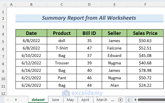
In this sample dataset there is sales data for a few products and the vendors that sold them in the months of March, April, May, and June.
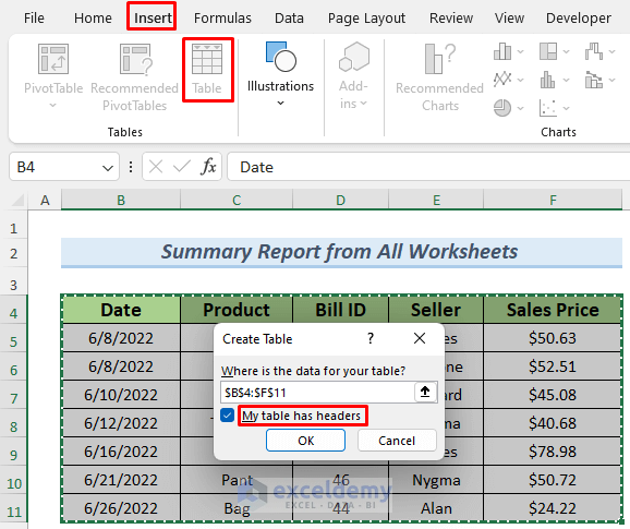
To convert this data to a table,
- In the Excel Ribbon, select Insert >> Table.
- A dialog box will appear. Make sure ‘My table has headers’ is checked, then click OK.
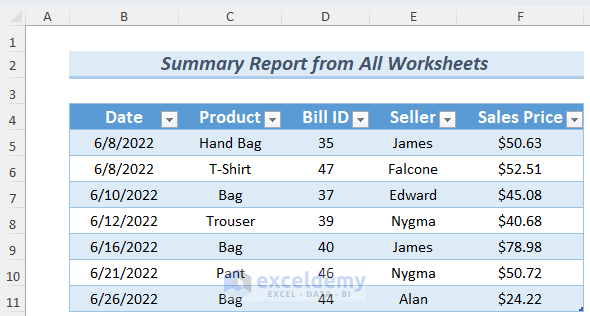
The data is then transformed into a table.
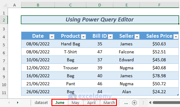
Method 1 – Using Power Query Editor and PivotTable to Create a Summary Table from Multiple Worksheets
We will be using the following sheets to create the summary table from multiple worksheets.
Steps:
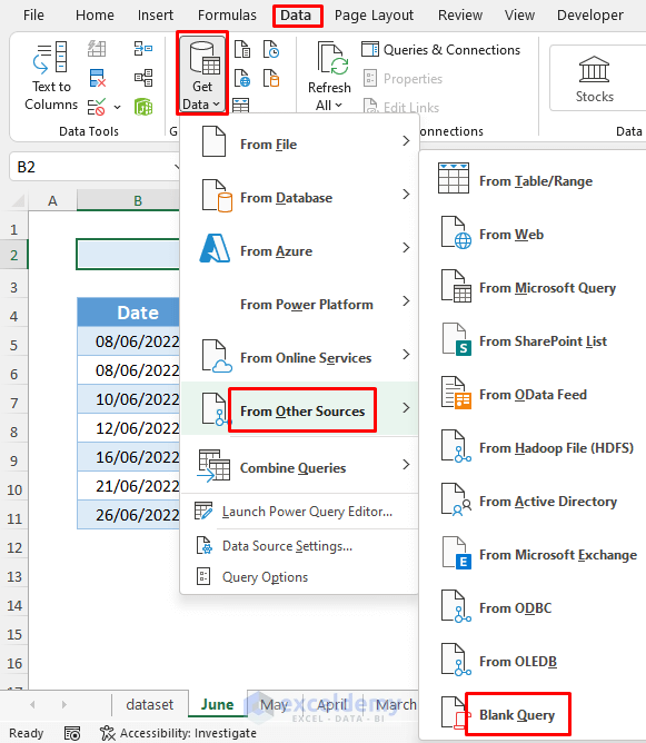
- Go to Data >> Get Data >> From Other Sources >> Blank Query.
- The Power Query Editor will open up.
- Give the Query a name. In this case, the name is Overall_Report.
- Press the ENTER button.
- In the Power Query formula bar, enter the following formula.
=Excel.CurrentWorkbook()
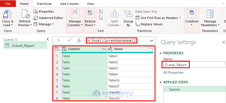
All of the workbook’s tables will be returned by the formula.
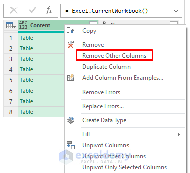
- To eliminate duplicates remove the second column using the Remove Other Columns command from the context menu by right-clicking on the header of the first column.
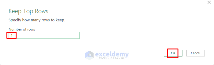
- Select Home >> Keep Rows >> Keep Top Rows.
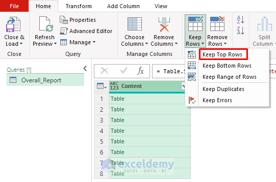
- The Keep Top Rows window will appear. Here four is entered since we will be working with the first four tables in this workbook.
- Click on the marked icon of the following image, uncheck Use original column name as prefix and click OK.
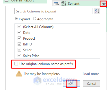
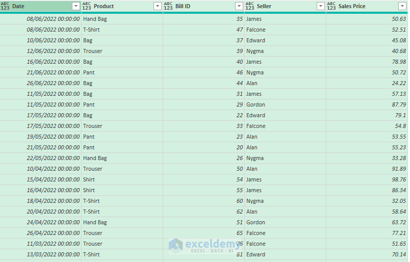
- The data from all sheets will then be combined.
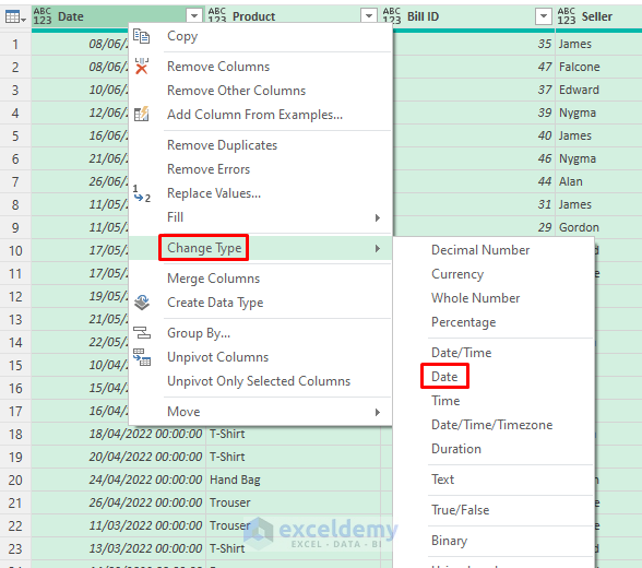
- The query might include some extraneous formatting, such as the date and time. To remove this, right click when selecting the Date column and then choose Change Type >> Date.
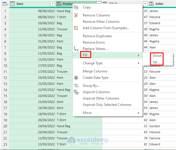
- If your data contains any blanks, select the columns that contain blanks and then Right-Click >> Fill. Select Down or Up as needed.
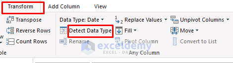
- Press CTRL+A and then go to Transform >> Detect Data Type. Although it’s not always essential, using this command is a good habit to get into when using the Power Query Editor.
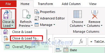
- Select Home >> Close & Load To…
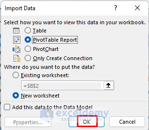
- The Import Data dialog box will appear. Select PivotTable Report, the sheet where you want the Pivot Table to be opened, and click OK.
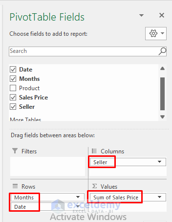
- The Pivot Table will appear on a new worksheet as we selected a New Worksheet in this instance. To view the worksheets’ compiled data, drag the Date range to the Rows Field, the Sales Price to the Values Field, and the Seller to the Columns Field.
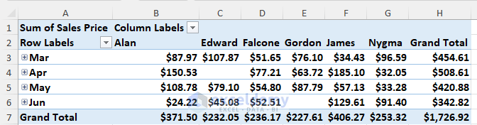
- You will see monthly and overall reports of the sales from March to June. You can also see seller-based sales records in your Pivot Table.
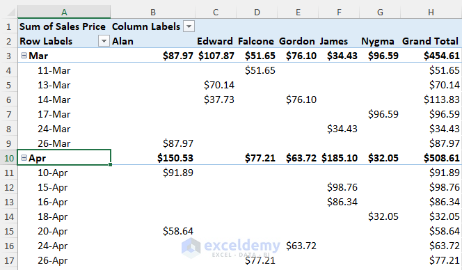
- Click on the Plus button next to the month name to learn more details about sales in that particular month.
You can create a Summary Table from Multiple Worksheets in Excel by using the Power Query Editor and Pivot Table.
Read More: How to Summarize Text Data in Excel
Method 2 – Applying 3D Reference to Create a Summary Table from Multiple Worksheets
Steps:
- Create a new sheet.
- Choose a cell to store the total Sales and use the formula below.
=SUM(June:March!F5:F11)
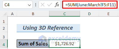
The formula uses the SUM function and sheet references to return the total Sales over the period March to June.
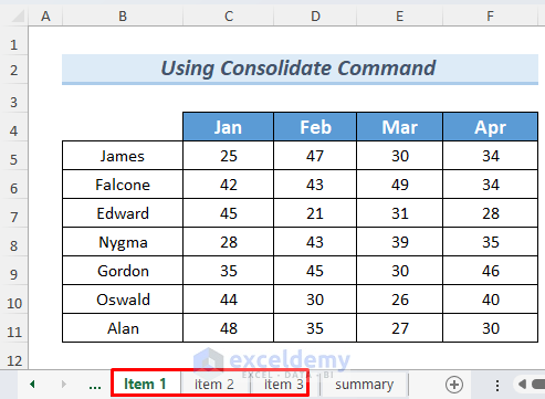
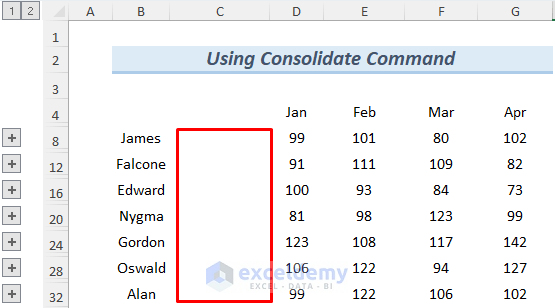
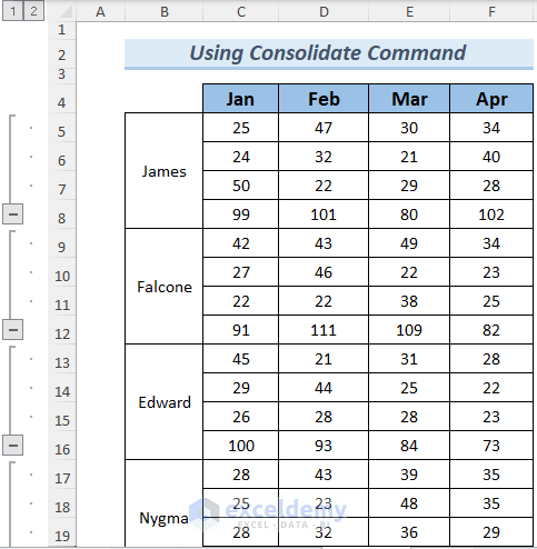
Method 3 – Using Consolidate Command to Create a Summary Table from Multiple Worksheets
The data shows how many sales of particular items have been made by the salesman over the months January to April.
Steps:
- Create a new sheet and select any cell where you want your combined data to start. Here a sheet named summary has been created.
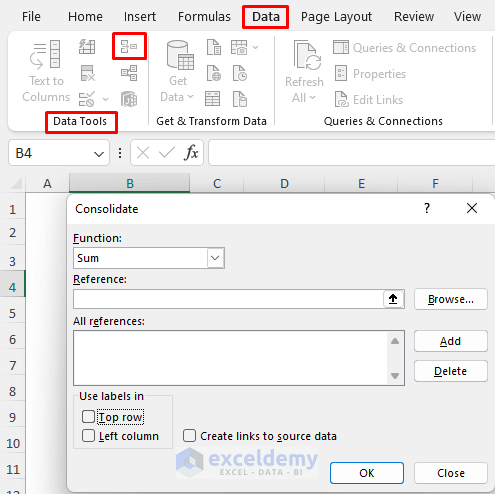
- Select Data >> Consolidate from the Data Tools group, and a Consolidate window will appear.
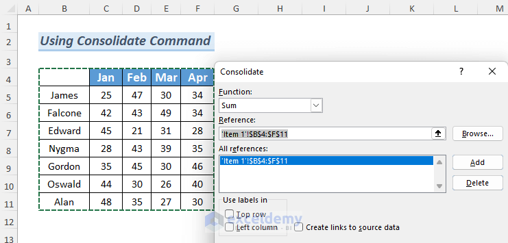
- Put the cursor in the Reference section and select the sheet where you put the data (in this case it’s Item 1).
- Select the range (B4:F11) which will be used to create the summary.
- Click Add.
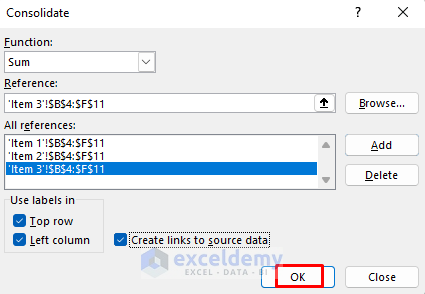
- Repeat to add the other ranges from Item 2 and Item 3.Check the options in the ‘Use labels in’ section.
- Click OK.
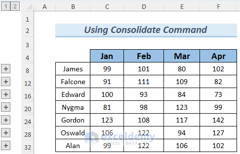
- In the new sheet the total sales quantity summary of each salesman for those items by month will be listed.
- Formatting will help make the summary table look better.
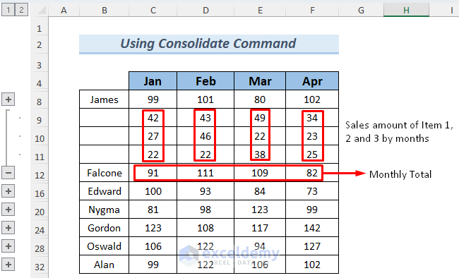
- The sales quantity by each item and month is hidden by these Plus icons. To see Falcone’s sales summary just click the Plus Icon beside his name.
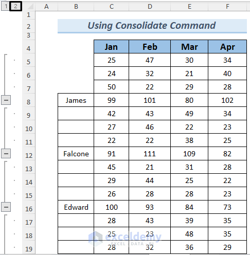
- To see detailed information, click on 2 button at the top-leftcorner of the sheet. Clicking on 1 will bring up the overall report again.
Merge the cells containing the salesman’s name to remove the unnecessary borderlines.
Read More: How to Summarize a List of Names in Excel
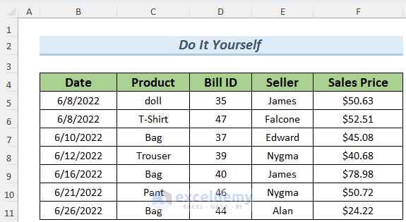
Practice Section
Download Practice Workbook
Related Articles
- How to Group and Summarize Data in Excel
- How to Create a Summary Sheet in Excel
- How to Make Summary in Excel From Different Sheets
- How to Summarize Data by Multiple Columns in Excel
- How to Summarize Data Without Pivot Table in Excel
- How to Summarize Subtotals in Excel
<< Go Back to Summarize Data In Excel | Data Analysis with Excel | Learn Excel
Get FREE Advanced Excel Exercises with Solutions!
