What Is 6 Sigma?
The term “6 Sigma” refers to a quality measurement that aims for absolute flawlessness. 6 Sigma is a methodical, computation approach for reducing errors in any process.
The calculation of 6 sigma involves two different approaches. One for discrete data, and another for continuous data.
Method 1 – Calculation of 6 Sigma with Discrete Data
Steps:
The sample dataset showcases the Number of Units, Number of Opportunities, and Total Number of Defects in the C4:C6 range.
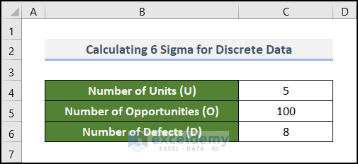
Here, U, O, and D represent the Number of Units, the Number of Opportunities, and the Number of Defects.
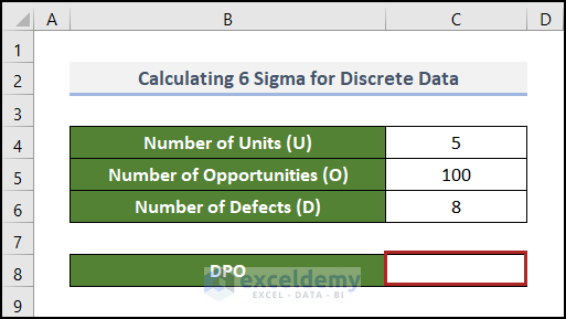
- To calculate the DPO, which is defects per opportunity from the previous data, use this generic formula.
- Create an output range in C8.
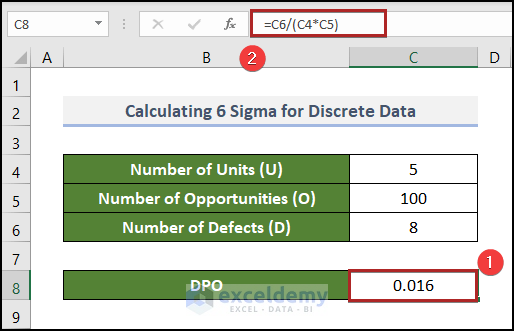
- Select C8 and enter the following formula.
=C6/(C4*C5)
- Press ENTER.
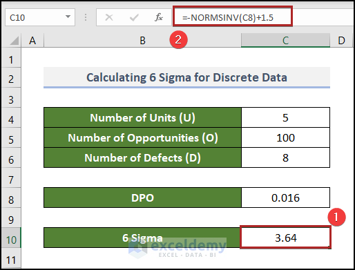
The universal formula to get the value of 6 Sigma from DPO is the following.
- Go to C10 and enter the formula below.
=-NORMSINV(C8)+1.5
The NORMSINV function returns the inverse of the normal distribution.
- Press ENTER.
Method 2 – Calculation of 6 Sigma With Continuous Data in Excel
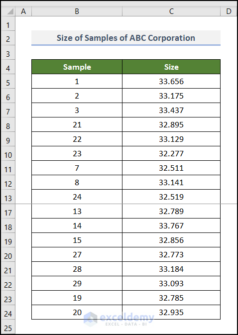
This is a continuous dataset, including the Sample numbers and their corresponding Sizes in columns B and C.
Steps:
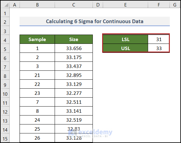
The LSL (Lower Specification Limit) and USL (Upper Specification Limit) were applied in this dataset. The ideal size is 32. A size variation of +/-1 is assumed. LSL and USL should be 31 and 33.
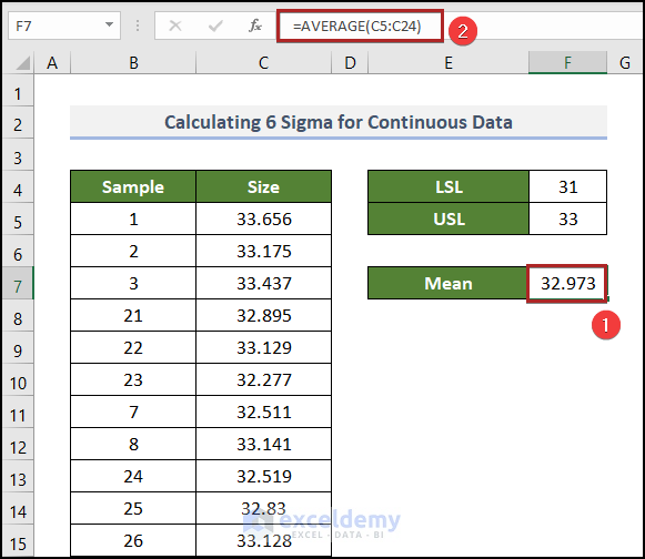
=AVERAGE(C5:C24)
Use the AVERAGE function to calculate the Mean. Here, C5:C24 represents the entire data range.
- Press ENTER.
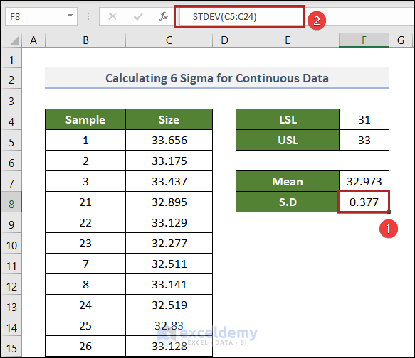
- Go to F8 and use the formula below.
=STDEV(C5:C24)
The STDEV function calculates the standard deviation.
- Press ENTER.
You calculate Cpu and Cpl for this dataset. Based on the system’s upper specification limit, the Cpu is an indicator of its conceivable competence. Cpl is based on the lower specification limit.
- Select F10 and enter the following formula.
=(F5-F7)/F8
- Press ENTER.
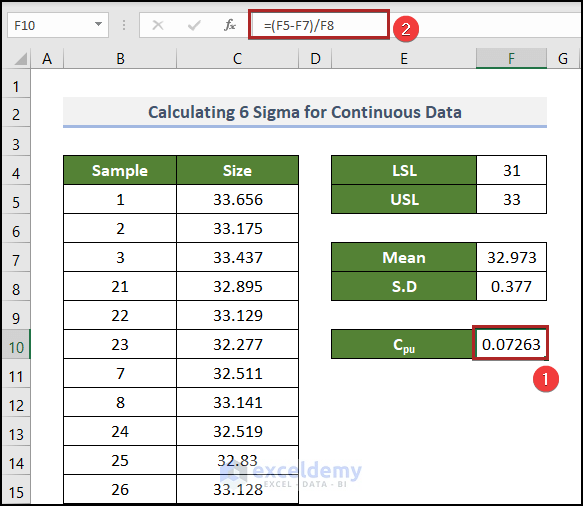
The value of Cpu is 0.07263.
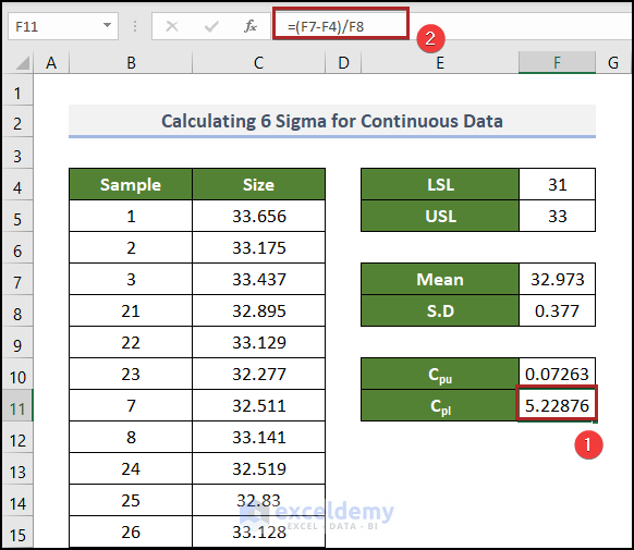
- Go to F11 and use the formula below.
=(F7-F4)/F8
- Press ENTER.
The 6 Sigma Value would be the minimum value between the values of Cpu and Cpl divided by the standard deviation.
- Go to F13 and enter the following formula.
=MIN(F10:F11)/F8
The MIN function returns the minimum value from a range of cells.
- Press ENTER.
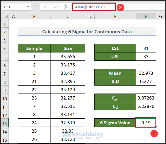
The value of 6 sigma for continuous data is displayed.
Read More:How to Calculate Sigma Level in Excel
How to Calculate 3 Sigma in Excel
Steps:
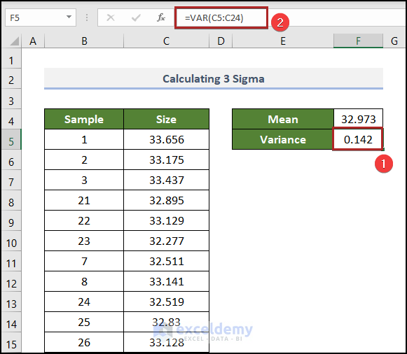
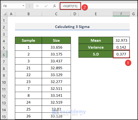
- Calculate the mean like before.
- Select F5 and enter the following formula.
=VAR(C5:C24)
The VAR function returns the variance of a sample taken from population data.
- Press ENTER.
- Select F6 and use the following formula.
=SQRT(F5)
The SQRT function returns the square root of any number. The standard deviation is found from the square root of the variance.
- Press ENTER.
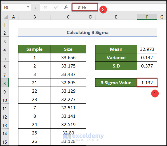
- Go to F8 and enter the formula below.
=3*F6
- Press ENTER.
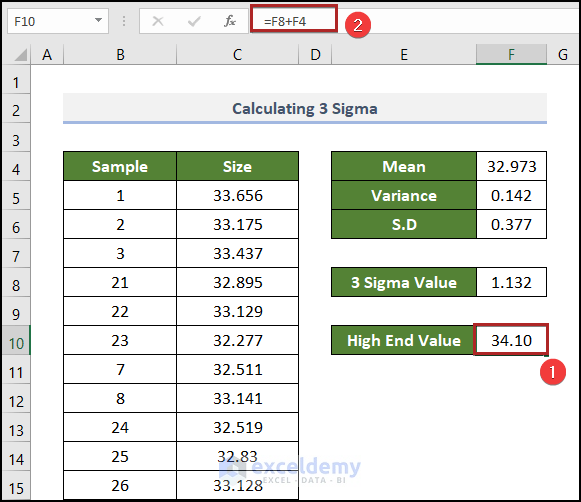
- Add the Mean value with the 3 Sigma Value to get the High End Value.
=F8+F4
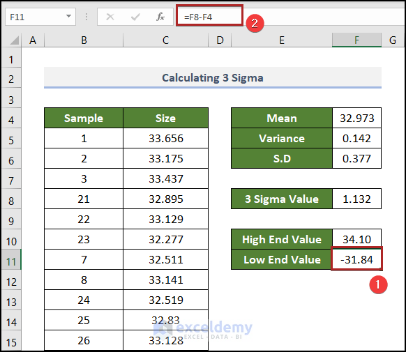
- You can extract the Low End Value by subtracting the Mean from the 3 Sigma Value.
=F8-F4
Practice Section
Practice here.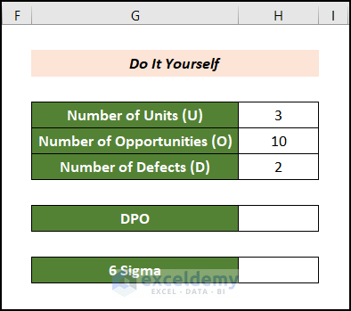
Download Practice Workbook
Download the following Excel workbook and practice.
Related Article
<< Go Back to Calculate Sigma in Excel | Excel for Statistics | Learn Excel
Get FREE Advanced Excel Exercises with Solutions!
