How to Calculate Sigma Level in Excel (2 Suitable Ways)

What Is the Sigma Level?

The Sigma level is a parameter to indicate the number of defects in 1 million opportunities. The sigma level indicates that if any industry produces 1 million products, how many defective products would be there. There are 6 sigma levels in the definition. Each one of them indicates different ranges of defects per million opportunities.

Sigma level 1: 697,672 defects in 1 million opportunities.
Sigma level 2: 308,770 defects in 1 million opportunities.
Sigma level 3: 66,811 defects in 1 million opportunities.
Sigma level 4: 6,210 defects in 1 million opportunities.
Sigma level 5: 233 defects in 1 million opportunities.
Sigma level 6: 3.4 defects in 1 million opportunities.

6 Sigma Calculation Formulas in Excel

We need the following values to find the sigma level.

Unit (U): This is the number of products taken into consideration for inspection.
Opportunity (O): This is the number of flaws possible in one unit.
Defect (D): This is the number of products that contain any number of flaws.
Defects per Unit (DPU): This is the ratio between the total number of defects and the total number of units.

DPU = ( D / U)

Defects per Opportunity (DPO): This is the average number of products per opportunity.

DPO = [D / (U*O)]

Defects per Million Opportunities (DPMO): This is the ratio of the number of defects in one million opportunities.

DPMO = (DPO * 1,000,000)

Rolled Throughout Yield (RTY): This is the percentage of products that is free of defects.

RTY % = (1-DPO)*100

Sigma Level: The most basic formula to calculate the Sigma Level in Excel is as follows:

Sigma Level = -NORMSINV(DPO)+1.5

How to Calculate the Sigma Level in Excel: 2 Suitable Ways

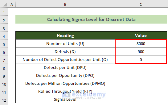
Method 1 – Calculate the Sigma Level for Discrete Data

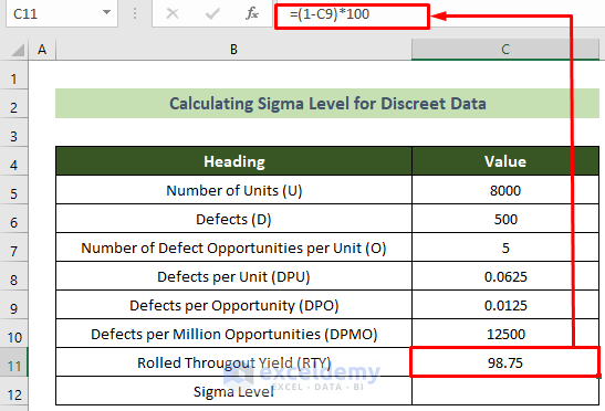
We need the inputs of the Number of Units, Defects, and Number of Defect Opportunities per Unit. We have these inputs in cells C5:C7.

We need to calculate the sigma level of this industry’s production scenario.

Steps:

Click on cell C8 and insert the following formula to calculate the Defects per Unit (DPU).

=C6/C5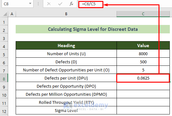

Click on cell C9, insert the formula below, and press the Enter key.

=C6/(C5*C7)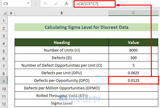

Click on cell C10 and insert the following formula to get the Defects per Million opportunities (DPMO).

=C9*1000000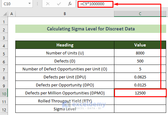

Click on cell C11 and insert the formula below.

=(1-C9)*100

Press the Enter key.

To calculate the sigma level, click on cell C11 and insert the following formula.

=-NORMSINV(C9)+1.5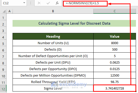

Method 2 – Calculate the Sigma Level for Continuous Data

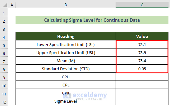
We will need the Lower specification Limit (LSL), Upper Specification Limit (USL), Mean (M), and Standard Deviation (STD) and the CPU, CPL, CPK values from the inputs. We have this data for the production in cells C5:C8.

Steps:

Click on cell C9 and insert the following formula to calculate the CPU value.

=(C6-C7)/(3*C8)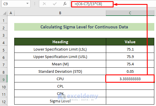

To calculate the CPL value, click on cell C10 and insert the formula below.

=(C7-C5)/(3*C8)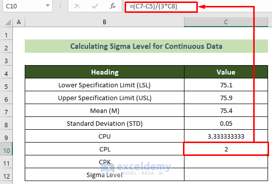

Click on cell C11 and insert the formula below.

=MIN(C9:C10)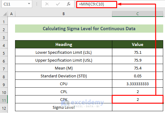

Click on cell C12 and insert the formula below to calculate the sigma level.

=3*C11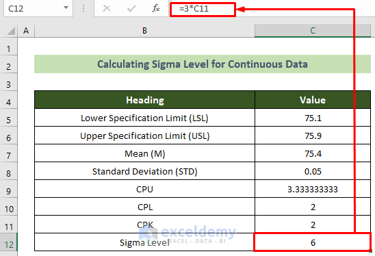

The sigma value for this production will be calculated as well.

Note:

You can also calculate the sigma level if you are given only one specification limit instead of both upper and lower. In that case, the given specification value’s CP will be the CPK value.

Download the Practice Workbook

Calculate Sigma Level.xlsx