
Conditional formatting turns a wall of numbers into something your eyes can scan in two seconds. Instead of reading every cell, you let color, icons, and bars do the work of flagging what needs attention. By applying the right rules, Excel can automatically highlight problem areas as soon as the data changes.
In this tutorial, we will show 5 conditional formatting tricks for spotting problems at a glance. These tricks will help you catch data-entry errors, outliers, status problems, and performance issues instantly.
1. Highlight Duplicates and Unique Values Instantly
Duplicates often signal copy-paste errors, double entries, or dirty data. Catching duplicate invoice numbers, repeated customer IDs, or accidental double entries is easy with conditional formatting.
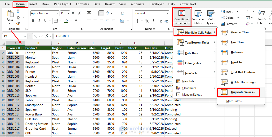
- Select your data range (e.g. a customer ID or invoice number column)
- Go to the Home tab >> select Conditional Formatting >> select Highlight Cells Rules >> select Duplicate Values
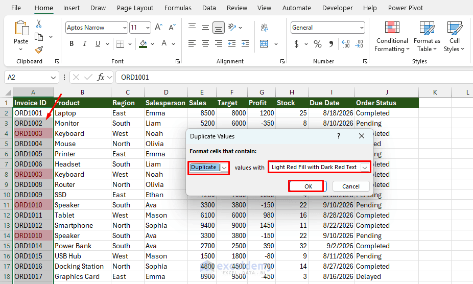
- Select Duplicate >> choose a fill color (red is the intuitive choice for “problem”)
- Click OK
Flag Duplicates Across Two Columns:
Sometimes you need to check if a value in Column A also appears in Column B (e.g. matching a “Shipped” list against an “Ordered” list).
Use a custom formula rule instead:
- Select the range to format
- Go to the Home tab >> select Conditional Formatting >> select New Rule
- Choose Use a formula to determine which cells to format
- Insert the following formula:
=COUNTIF($B$2:$B$500, A2) > 0
- Click Format to set your fill color
- Click OK
This is more flexible than the built-in duplicate checker because it works across ranges, not just within one column.
2. Use Color Scales to Find Unusually High or Low Values
Sometimes there is no fixed threshold for identifying a problem. You simply want to see which values are unusually high or low compared with the rest of the dataset. Color scales are great for spotting patterns across a grid, like monthly sales by region, but the default 3-color scale often washes out real differences.
- Select your data range
- Go to the Home tab >> select Conditional Formatting >> select Color Scales
- Select a suitable three-color scale
- Useful variations:
- Red-Yellow-Green for performance (low = problem)
- White-Blue for volume (darker = higher)
- Custom midpoint based on a target value
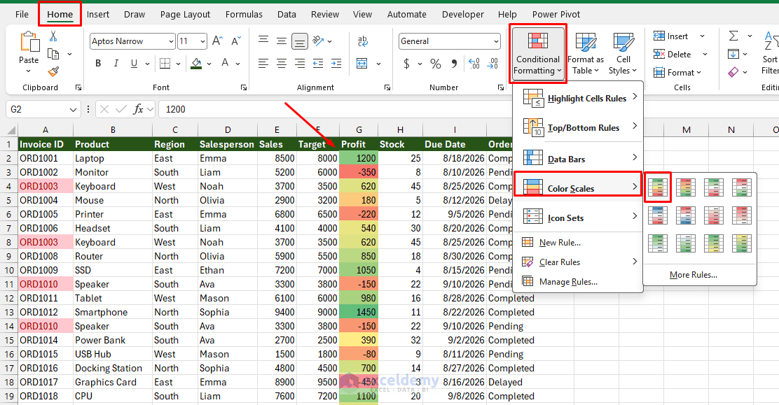
Excel applies different colors based on the relative size of each value. You can now identify low-stock and high-stock products without reading every number individually.
Customize the Scale:
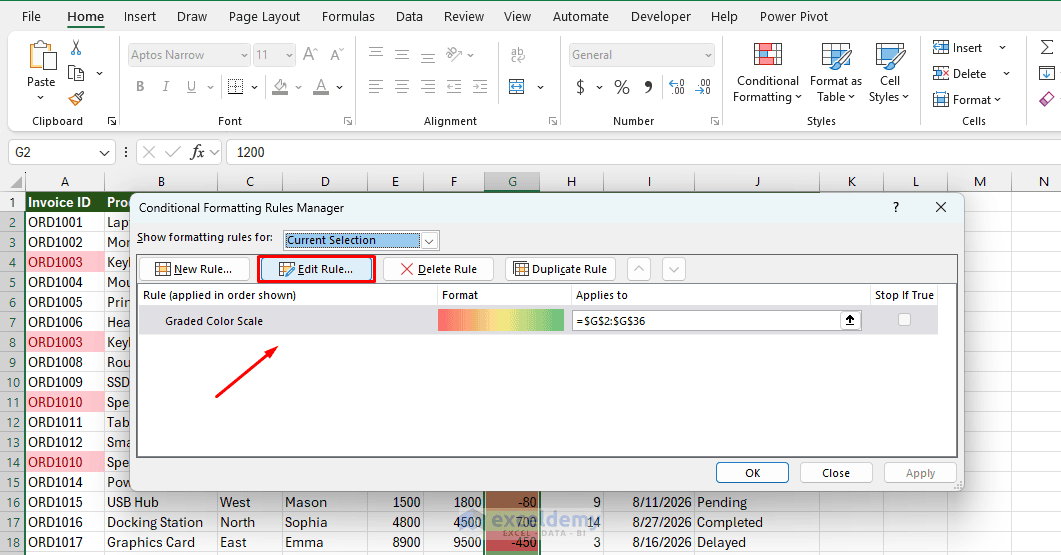
- Select your numeric range where you applied formatting
- Go to the Home tab >> select Conditional Formatting >> select Manage Rules
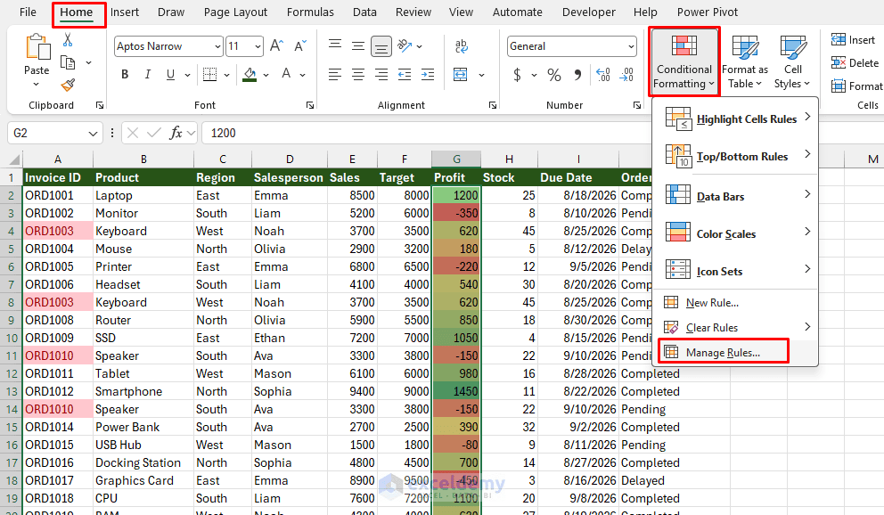
- Select the Color Scale rule >> click Edit Rule
- Define your own minimum, midpoint, and maximum values
- Minimum: 0
- Midpoint: 750
- Maximum: 1500
- Click OK
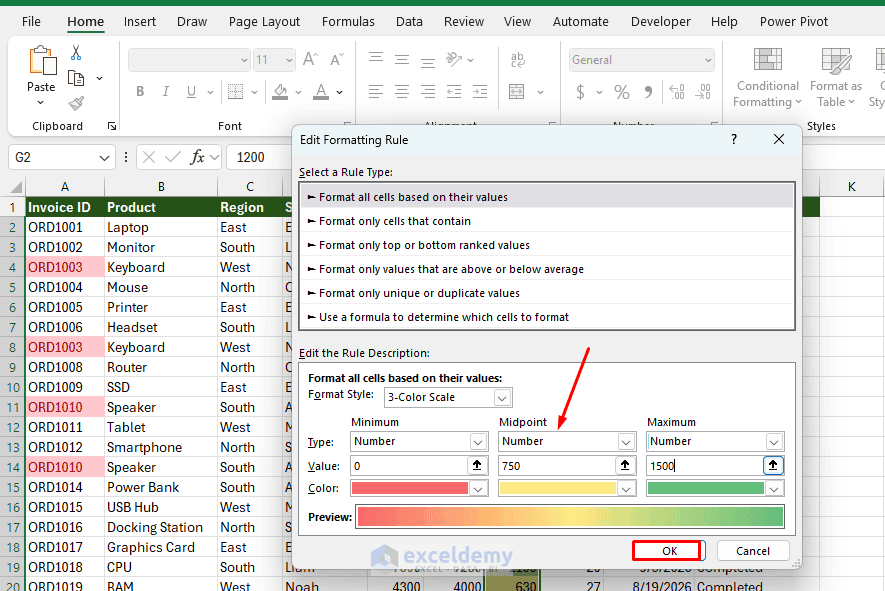
This makes the formatting more meaningful for your actual inventory levels.
3. Data Bars That Reveal Outliers, Not Just Magnitude
Data bars are often used lazily — just applied and left alone. But their real power is in spotting outliers when you tweak the settings.
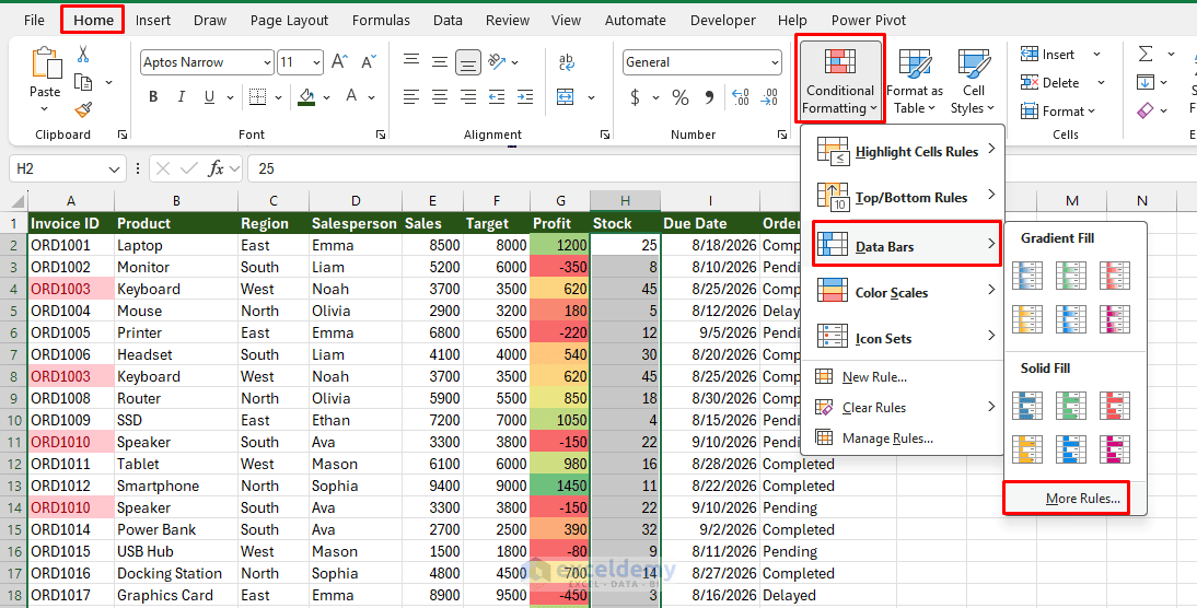
- Select your numeric range
- Go to the Home tab >> select Conditional Formatting >> select Data Bars >> select More Rules
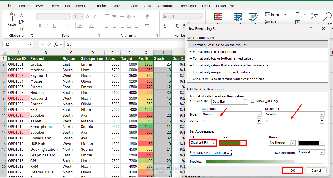
- Under Bar Appearance, set:
- Fill: Gradient Fill (draws the eye better than solid)
- Negative Value and Axis: Set a distinct color (e.g. red) for negatives — this instantly separates over-budget items from under-budget ones in a variance column
- Under Minimum/Maximum, switch from “Automatic” to Number and set fixed values
- Min = 0
- Max = 50
- Click OK
You will get your customized data bars.
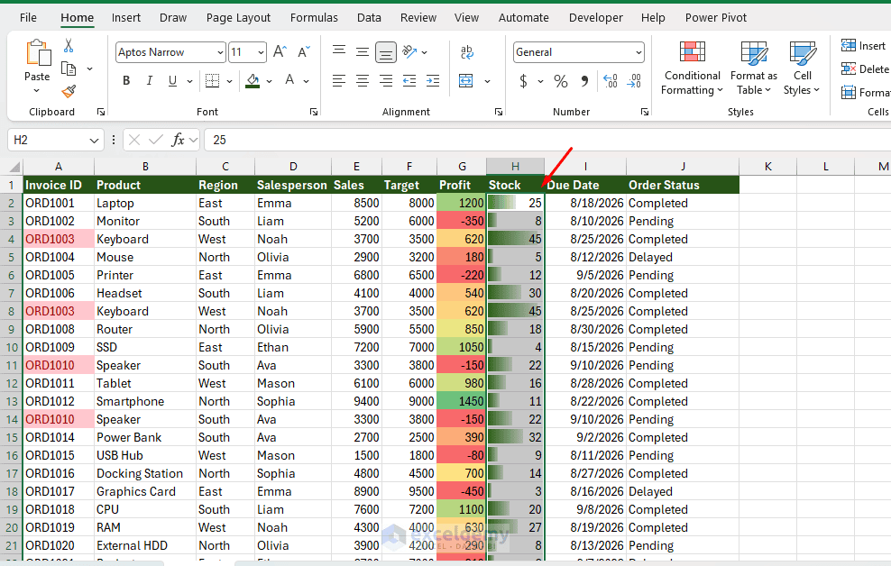
Why fixed min/max matters: With “Automatic,” Excel rescales the bars every time your data changes, so a bar that looks “average” today might look “huge” tomorrow, even though the underlying number didn’t change relative to your real targets. Fixing the scale means a long bar always means “large relative to my actual business threshold,” which is what makes outliers reliably jump out.
4. Flag Negative Values Automatically
Negative profit, cash flow, or variance values usually deserve immediate attention.
- Select the cell range
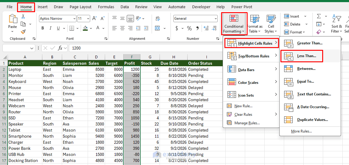
- Go to the Home tab >> select Conditional Formatting >> select Highlight Cells Rules >> select Less Than
- In Format cells that are LESS THAN enter: 0
- Choose the formatting you want
- Click OK
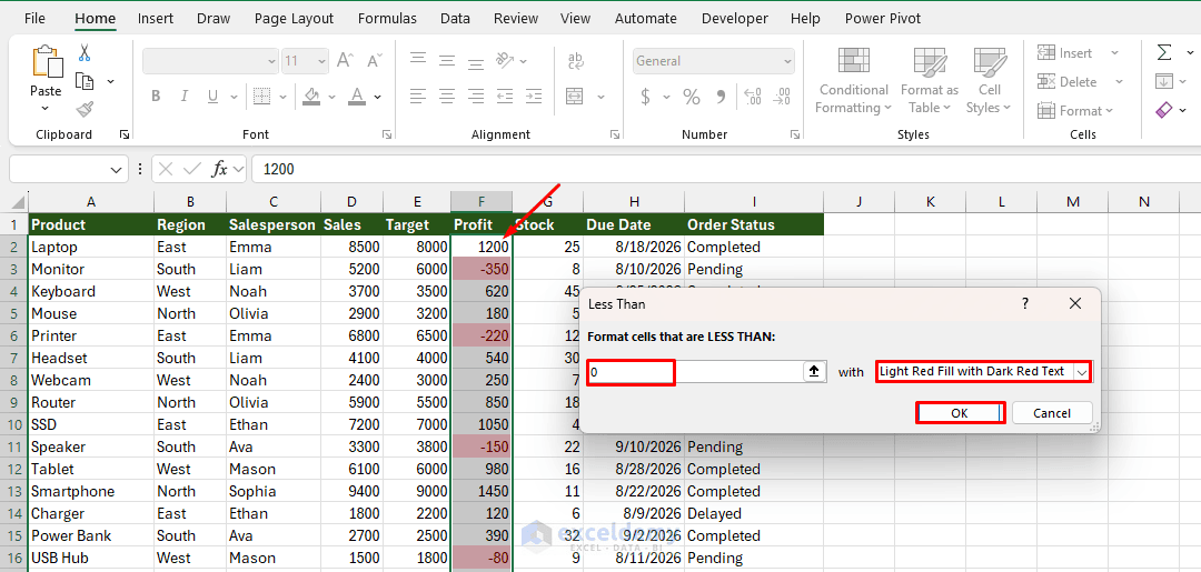
All negative profits will now stand out automatically.
Alternative: Highlight the Entire Row
You can make the problem even easier to spot by highlighting the entire record.
- Select your data range
- Create a formula-based rule, and enter:
=$F2<0
The $ locks the rule to the Profit column while allowing Excel to evaluate each row separately.
5. Formula-Driven Rules to Highlight Entire Rows
Highlighting a single problem cell is useful, but highlighting the whole row makes it far easier to scan a long list — especially when the problem column isn’t the one you’re currently looking at.
Highlight an entire row when a task’s due date has passed and the status isn’t “Complete”.
- Select the full data range
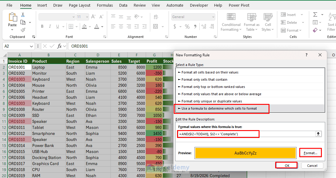
- Go to the Home tab >> select Conditional Formatting >> select New Rule
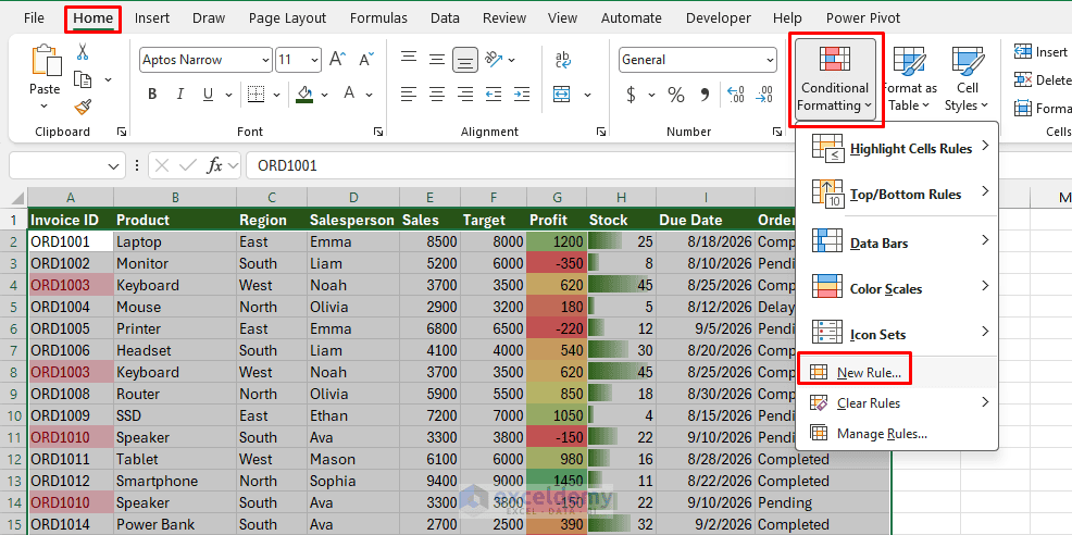
- Choose Use a formula to determine which cells to format
- Enter (assuming Due Date is in column I and Status is in column J):
=AND($I2<TODAY(), $J2<>"Complete")
- Set a fill color (light red or orange works well)
- Click OK
Now entire rows are highlighted where a task’s due date has passed and the status isn’t “Complete”.
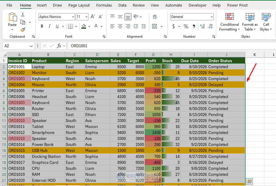
Key Detail: The $ before the column letter ($I2, $J2) locks the column reference but lets the row adjust — this is what makes the rule apply correctly across every row in your selection instead of always checking row 2.
Common “Problem-Spotting” Formulas:
| Goal | Formula Example | What it highlights |
| Entire row when status = “Overdue” | =$E2=”Overdue” | Whole row for overdue items |
| Stock below reorder level | =$C2<$D2 | Rows where Qty < Reorder Point |
| Dates more than 30 days old | =$B2<TODAY()-30 | Stale records |
| Negative or zero values | =$F2<=0 | Problem values |
| Text that fails a check | =AND($G2<>””,$G2<$H2) | Specific business-rule violations |
Pro Tip: Always write the formula relative to the top-left cell of your selection. Excel will adjust it for every other cell.
Quick Implementation Tips
- Order Matters: Rules are evaluated from top to bottom. Put the most specific rules higher in the list.
- Stop If True: Use this checkbox when a cell should only get one format.
- Manage Rules: Home → Conditional Formatting → Manage Rules is your control center. You can edit, delete, or change the order of rules easily.
- Performance: On very large ranges (tens of thousands of rows), prefer simple rules over complex formula-based ones when possible.
- Copy Formatting: Use the Format Painter or “Paste Special → Formats” to apply the same rules to other sheets.
Conclusion
With these five conditional formatting tricks, you can turn a normal worksheet into a visual monitoring system. Start with the ones that match the problems you see most often — duplicates and threshold breaches are usually the highest-ROI places to begin. Because conditional formatting updates automatically when the underlying values change, problem areas remain visible without requiring you to repeatedly inspect the worksheet manually.
Get FREE Advanced Excel Exercises with Solutions!