What Is the Task Pane in Excel?
The Task Pane is a standard interface element in Microsoft Office applications, including Word, Excel, PowerPoint, and Outlook.
List of Available Task Panes in Excel 365
The Task Panes are listed below:
Accessibility Checker – checks the file condition.
Actions – is utilized for individualized document creation (Excel and Word). Inaccessible via the user interface.
Clipboard – a collection of features that allow users to copy and paste data between various Office programs.
Data Selector – assists in picking the best form of related data.
Document Recovery -when Excel restarts following a crash, this window opens automatically. It shows the last saved your work, so you can restore the file.
Format Chart Element – is used to modify charts and chart elements.
Analyze Data – is known as Ideas.
Navigation – finds items in your workbooks like tables, graphs, PivotTables, and pictures.
Selection – contains the Home tab, Editing, Find & Select.
Thesaurus – is a synonyms and antonyms dictionary.
Translator – helps to translate.
Watch Window – in the watch window, you can Add the Formulas tab, with Formula Auditing.
How to Add Task Pane Add-ins in Excel
Steps
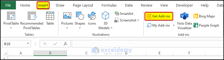
- To add an add-in, go to the Insert tab and click Get Add-Ins.
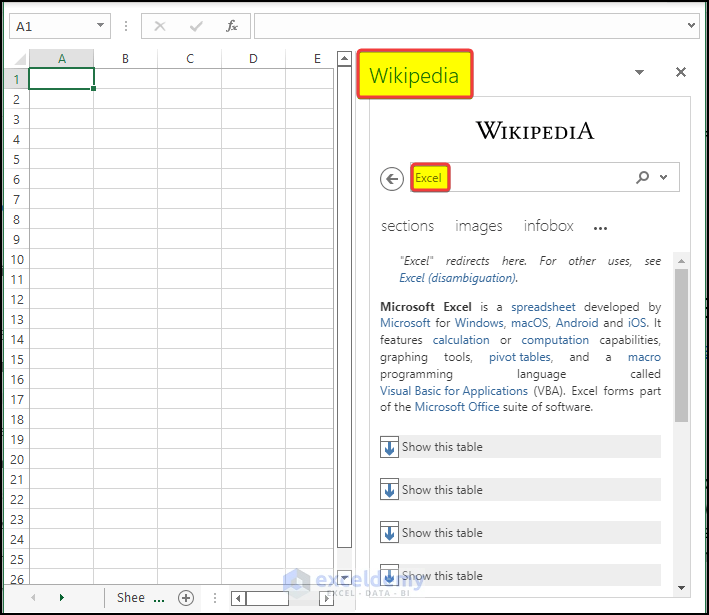
- In Microsoft Add-ins Store, search for Wikipedia.
- Click “Add“

Wikipedia is added to the worksheet. There is a pane on the right side of the worksheet. Use it to search for information.
How to Show a Task Pane in Excel
Some commands in Excel will respond automatically with Task Panes. For example:
Steps
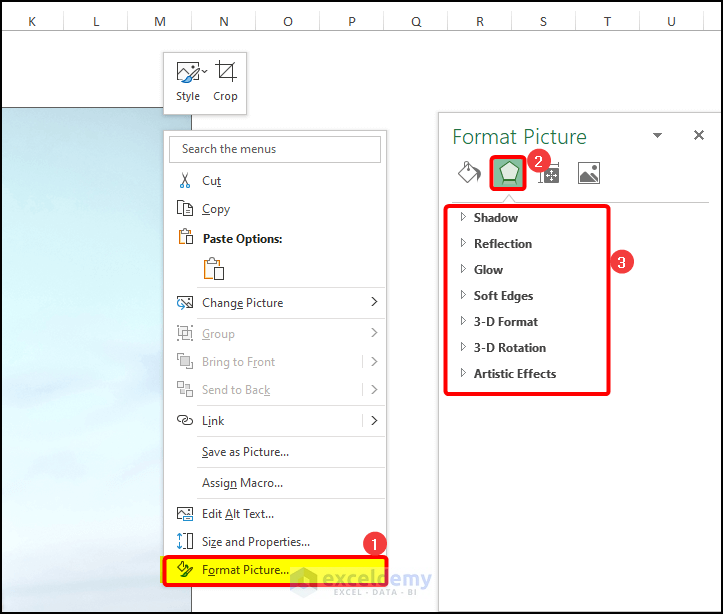
- Select an Image and right-click it.
- Click Format Pictures.
- The Picture Task Pane will open.
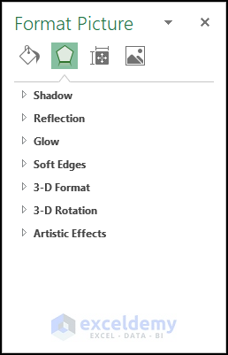
- In the Picture Task Pane, we can see different options in Effects.
If you work with a chart, you can access a chart-related Task Pane containing commands for every element within the chart:
- The Format Picture Task Pane has four icons- Fill & Line, Effects, Size & Properties, and Picture.
- The names are shown when you hover your mouse pointer over the icons. Click an icon and you will find a command list.
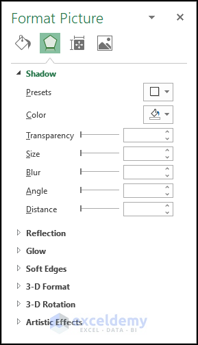
- Click Shadow and you will see different style options.
How to Use a Task Pane in Excel
1. Navigating Within a Task Pane in Excel
There’s no OK button in a Task Pane.
Steps
- Click Close (X) in the upper-right corner.
- Press F6 to activate the Task Pane. Use the tab key, the arrow keys, the spacebar, and other keys to navigate within the Task Pane.
2. Setting Position of Pane in Excel Worksheet
By default, the Task Pane is placed on the right side of the Excel window. To move it, click the title bar and drag it. You can also use ‘Task Pane Options’ and choose: Move, Size, and Close.
3. Setting a Task Pane in a Different Place
Excel stores the last position of your Task Pane.
How to Open a Research Task Pane in Excel
Steps
- Press Alt+select any cell in the worksheet.
- The Research pane will be displayed on the right side of the sheet.
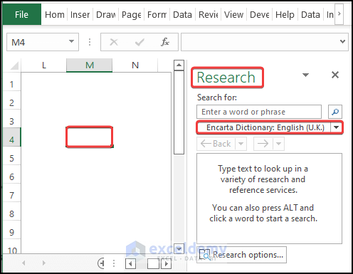
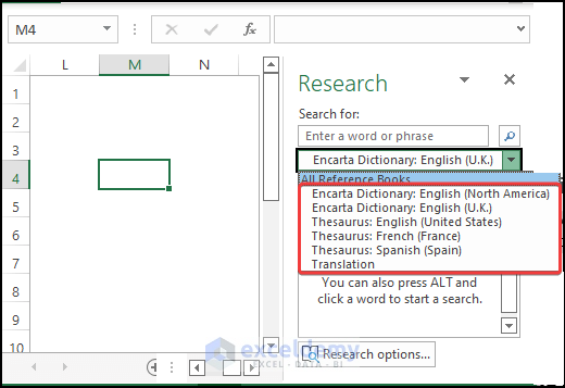
You can see the dictionary or language options and look up keywords.
How to Disable the Research Task Pane in Excel
Steps
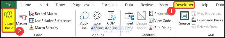
- Go to the Developer tab and click Visual Basic. (If you don’t have it, you have to enable the Developer tab). You can also press ‘Alt+F11’ to open the Visual Basic Editor.
- Click Insert > Module.
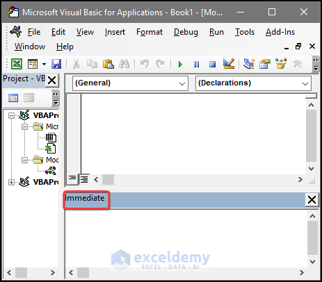
- In the Module editor window, press Ctrl+G.
- The Immediate window will be displayed below the editor window.
- Use the following code and press enter.
Application.CommandBars("Research").Enabled = False
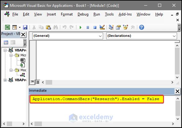
The research pane is no longer displayed.
How to Open the Alt Text Task Pane to Add or Modify Alt Text in Excel
Steps
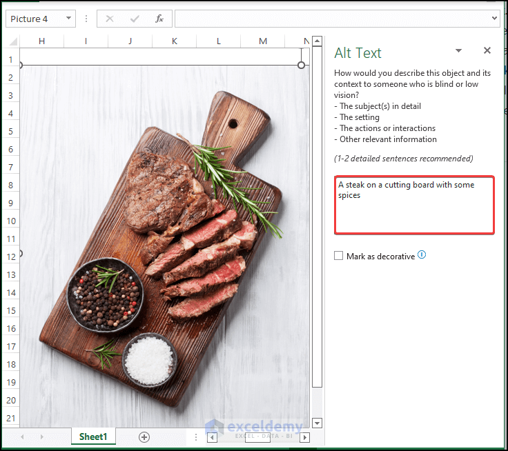
- To view an Alt text of an image, add it in Insert Image.
- Right-click the image and click Edit Alt Text.
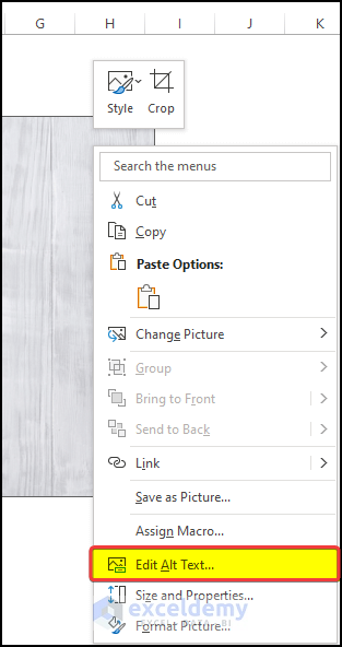
The Alt Text side panel will be displayed.
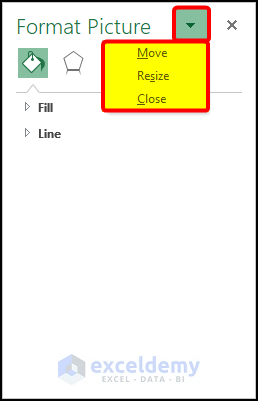
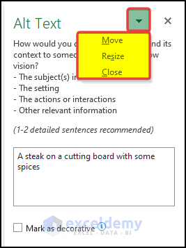
- To move the Alt text pane, click the downward arrow in the pane.
- Click Move and drag the pane. Place it in another location.
- You can also resize the pane by clicking Resize.
- To close the pane, click Close.
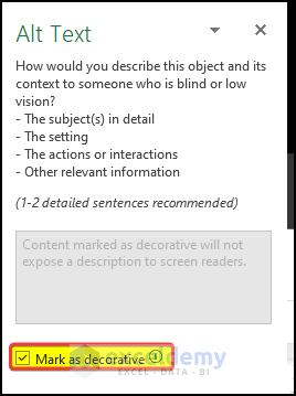
- Make the text decorative by checking Mark as decorative.
- People with no access to the document cannot read the Alt text.
How to Use an XML Source Task Pane to Map XML Elements
Steps
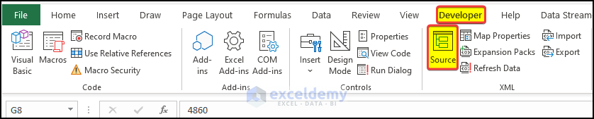
- To show the XML source pane, load the XML file into the worksheet: click Import in the Developer tab.
- Select the file.
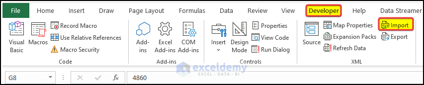
- To see the Task Pane of that file, click Source in the Developer tab.
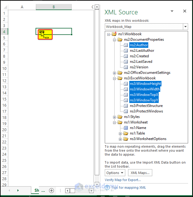
- The Task Pane will be displayed on the right side of the sheet.
- The structure and layers of the XML file will be shown in different folders.

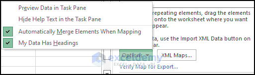
- You can check these Options:
Preview Data in Task Pane – shows sample data in the component list.
Hide Help Text in the Task Pane – Displays contextual help text.
Automatically Merge Elements When Mapping – the content of an XML list.
My Data Has Headings – column headings.
Hide Borders of Inactive Lists – the margins of cells outside the XML element list will not be shown.
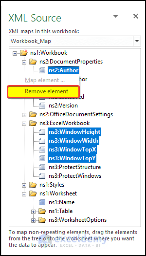
Mapping Elements
To establish a connection between a cell and an XML:
- Go to Data > XML > Source.
- Click the items you want to map inside the XML task window and they will be displayed in your worksheet.
- To select several, non-contiguous components, click each one of them pressing Ctrl.
- Drag the element(s) to the worksheet.
- Each mapped element in the Source pane is bold in Excel.
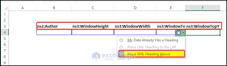
- Choose how to handle labels and column titles.
How to Use the Document Recovery Task Pane in Excel
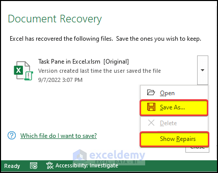
Steps
- Open Excel.
- The recovery pane will show recovered files.
- You can also see the repairs done on the file.
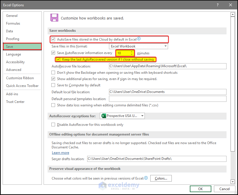
To enable autosave in the settings menu and keep the time period between the autosave minimal.
- Click File > Options.
- Click Save.
- Check Keep the Last AutoRecovered version if I close without saving.
- Check Save AutoRecovered information every box and set an autosave time interval.
- Click OK.
<< Go Back to Excel Parts | Learn Excel
Get FREE Advanced Excel Exercises with Solutions!
