Having up and down arrows in the proper places of datasets makes them more presentable and visually pleasing. Excel’s default arrow formatting inserts three types of arrows. But suppose we only want to use up and down arrows, for example to represent the upward or downward direction of prices. We can accomplish this using conditional formatting.
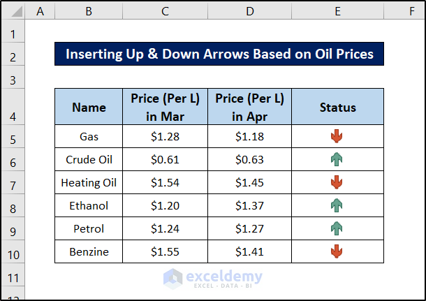
Example 1 – Inserting Up and Down Arrows Based on Oil Prices
Consider the following dataset:
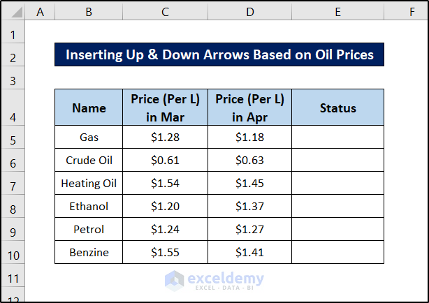
For some entries, the price has gone up. And for others, the price has gone down.
Let’s represent this movement with up and down arrows using the SIGN function (which takes a number as an argument and returns a negative or positive one depending on the sign of the argument, zero if the input is zero, and an error for non-numeric values) and conditional formatting.
Steps:
- Select cell E5.
- Enter the following formula:
=SIGN(D5-C5)
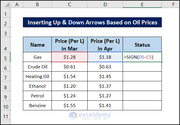
- Press Enter.

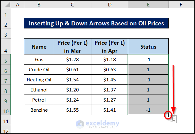
- Select the cell again and click and drag the fill handle icon to the end of the column to replicate the formula for the rest of the cells.
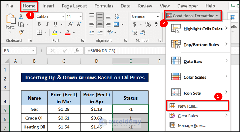
- Select the range if it is not selected already.
- Go to the Home tab on your ribbon.
- Select Conditional Formatting from the Styles group.
- Select New Rule from the drop-down menu.
The New Formatting Rule box will open up.
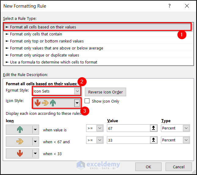
- Select Format all cells based on their values in the Select a Rule Type section.
- Select Icon Sets as the Format Style under Format all cells based on their values.
- Select Arrows as the Icon Style.
- Select Number in both the Type drop-downs as shown in the figure.
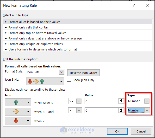
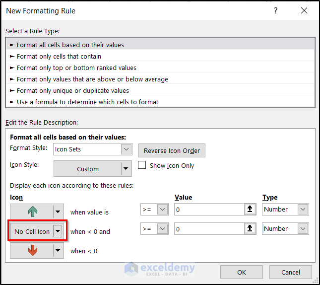
- Select No Cell Icon for the when <0 and option.
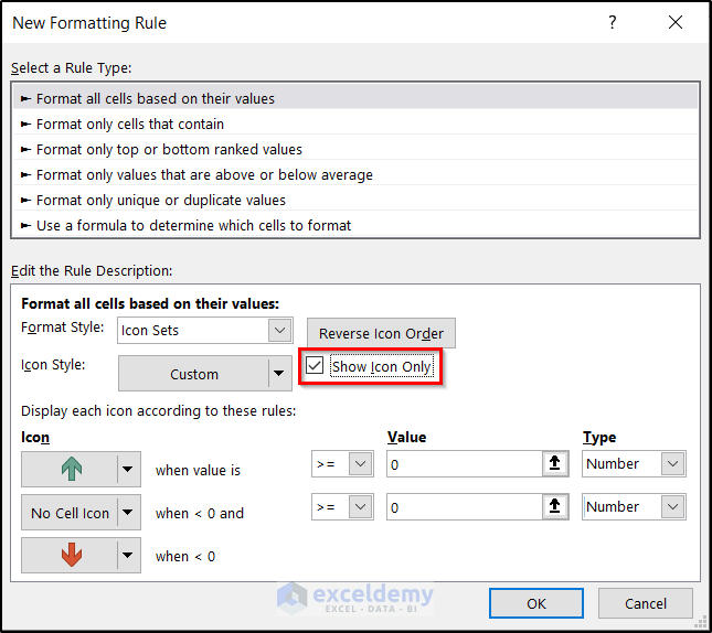
- You can also check/uncheck the Show Icon Only option, depending on whether you want to show the value beside the icon or not. We are opting not to choose the numbers to show.
- Click on OK.
The dataset will change to something like this.
Read More: How to Add Up and Down Arrows in Excel
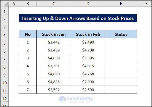
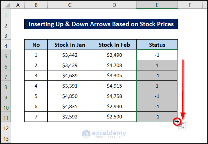
Example 2 – Inserting Up and Down Arrows Based on Stock Prices
Here is a dataset of stock prices in different periods.
In a similar fashion to Example 1 above, we can indicate the upward or downward motion of the stock price with up and down arrows.
Instead of using the SIGN function, we’ll use the IF function to determine the increase or decrease in price. The IF function tests a condition and returns an output if the result is true, and optionally another output if the result is false.
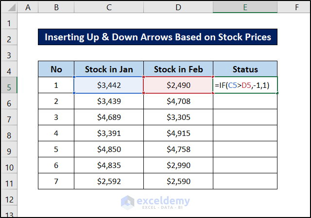
Steps:
- Select cell E5.
- Enter the following formula in it:
=IF(C5>D5,-1,1)
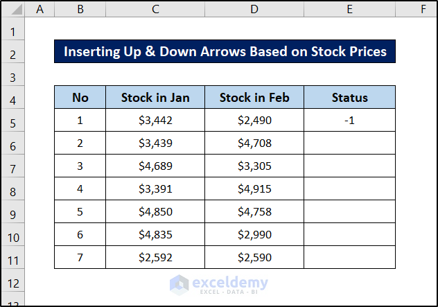
- Press Enter.
- Select the cell again and click and drag the fill handle icon bar to the end of the column to replicate the formula for the rest of the cells.
- Go to the Home tab while the column is still selected.
- Click on Conditional Formatting from the Styles group.
- Select New Rule from the drop-down menu.
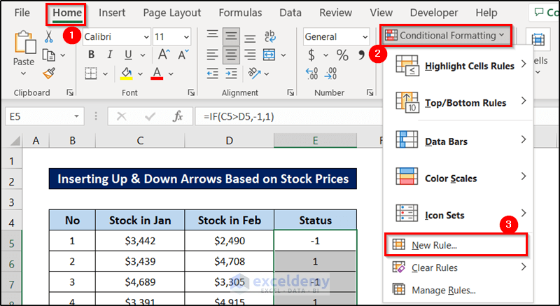
The New Formatting Rule box will open up.
- Select Format all cells based on their values in the Select a Rule Type section.
- Select Icon Sets as the Format Style under Format all cells based on their values.
- Select Arrows as the Icon Style.
- Select Number in both the Type drop-downs as shown in the figure.
- Select No Cell Icon for when <0 and option.
- You can also check/uncheck the Show Icon Only option, depending on whether you want to show the value beside the icon or not. We are opting not to choose the numbers to show.
- Click on OK.
The arrows will appear in the cells, replacing the numbers.
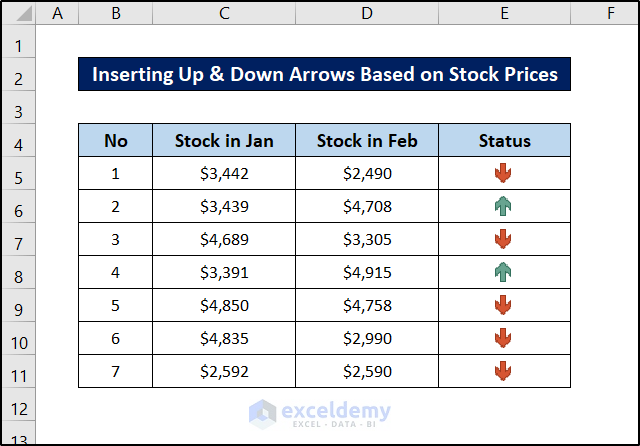
The Arrows created in this method are dynamic, and will change as values change in the source cells.
Read More: How to Add Trend Arrows in Excel
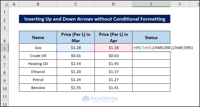
How to Insert Up and Down Arrows Without Conditional Formatting in Excel
The methods above insert up and down arrows using conditional formatting. We can also use a combination of the IF function and the CHAR function to achieve a similar result without using conditional formatting.
The IF function tests a condition and returns an output if the result is true, and optionally another output if the result is false. The CHAR function takes only a number as the argument and returns a character based on the number it represents.
Steps:
- Select cell E5.
- Enter the following formula in it:
=IF(C5>D5,CHAR(200),CHAR(199))
- Press Enter.
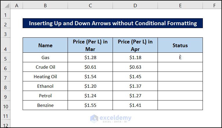
The exact output may not display yet.
- Select the cell again. Then click and drag the fill handle icon to the end of the column to replicate the formula for the rest of the cells.
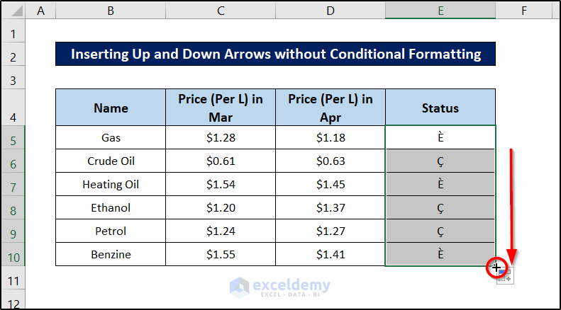
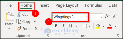
Now you need to change the font style of the desired cells where you want to insert up and down arrows.
- Select the cells first.
- Go to the Home tab and select Wingdings 3 as the font style from the Font group.
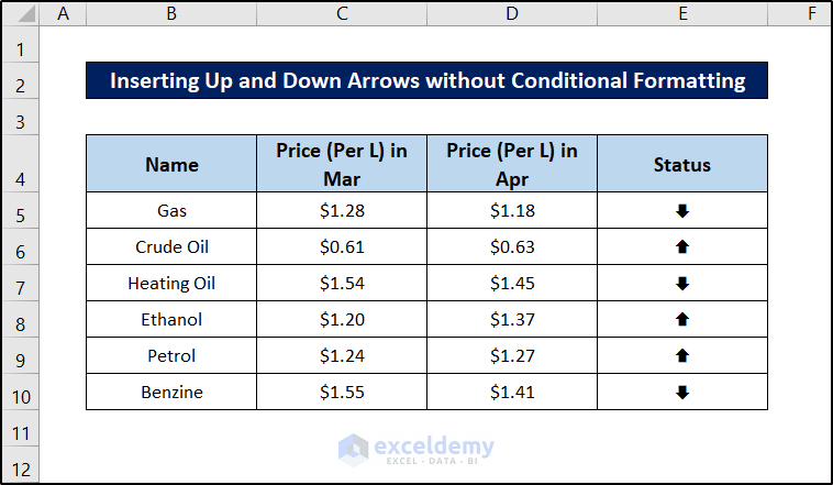
The cell values will change into arrow signs.
Download Practice Workbook
Related Articles
- How to Insert Red Arrow in Excel Cell
- How to Insert Curved Arrow in Excel
- How to Use Blue Line with Arrows in Excel
- How to Remove Tracer Arrows in Excel
- Double Headed Arrow in Excel
- How to Show Tracer Arrows in Excel
- How to Insert Trend Arrows Based on Another Cell in Excel
<< Go Back to Arrows in Excel | Excel Symbols | Learn Excel
Get FREE Advanced Excel Exercises with Solutions!
