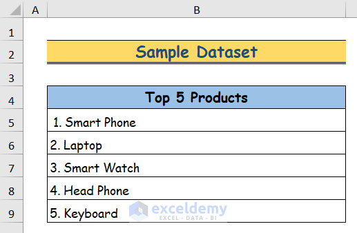
Let’s use the following dataset to illustrate the methods of inserting a tab in a cell.
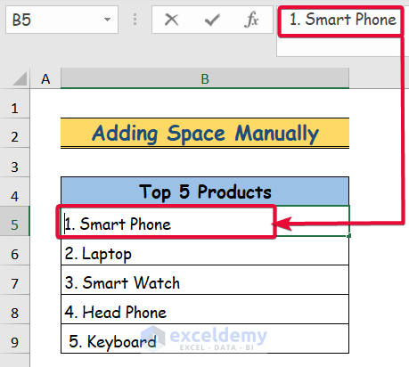
Method 1 – Adding Spaces Manually
Steps:
- Double-click on the B5 cell.
- Take the cursor to the leftmost side of the cell.
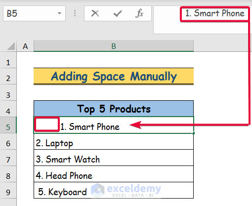
- Press the space button multiple times according to how much space you need. We will press it ten times in a row.
- A “tab” is inserted in front of the value in the cell.
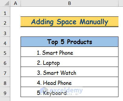
- Repeat for the rest of the cells.
Method 2 – Applying the Increase Indent Command
Steps:
- Select the cell you want to indent.
- Go to the Home tab in the ribbon.
- Select the Alignment group.
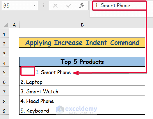
- Click on the Increase Indent command until you get a result you need.
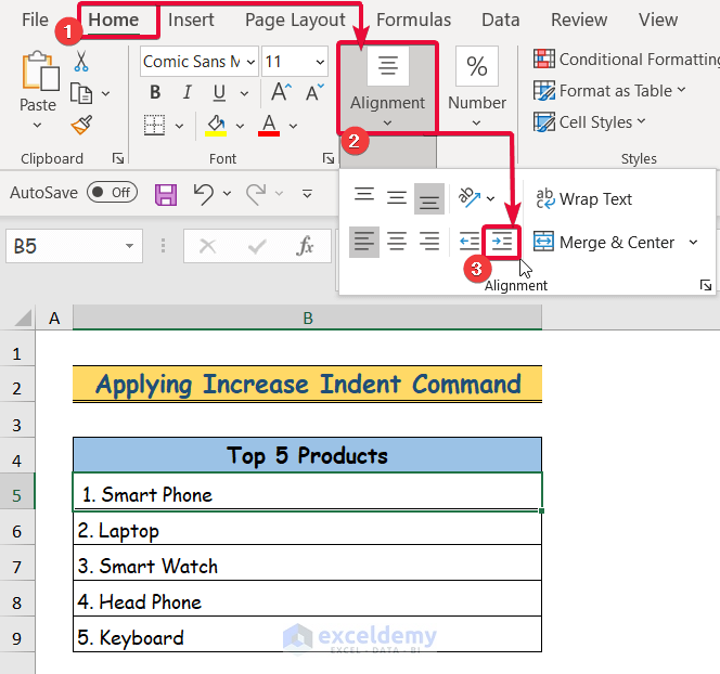
- You will find your data tabbed.
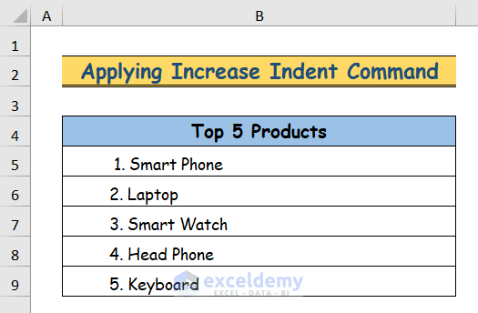
- Repeat the process for the rest of the dataset.
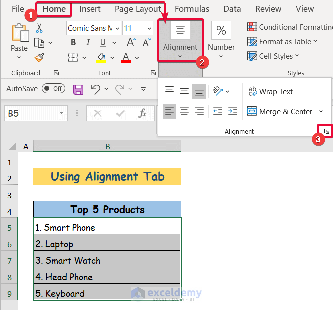
Method 3 – Using the Alignment Tab
Steps:
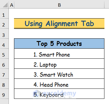
- Select the cells in the dataset. We will select the cells in the range (C5:C9).
- Choose the Home tab in the ribbon.
- Go to the Alignment group.
- Select the tiny anchor to the bottom right of the Alignment group.
- The Alignment tab of the Format Cells dialogue box will be on the screen.
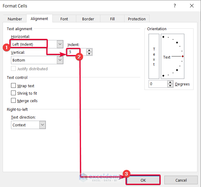
- In the Alignment tab, under the Horizontal option, make the text alignment Left(Indent).
- Under the Indent option, select the number of indents. We opted for 5.
- Click OK.
- The data will have a tab before them.
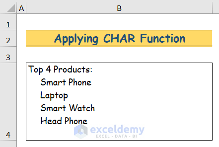
Method 4 – Applying CHAR and REPT Functions
Steps:
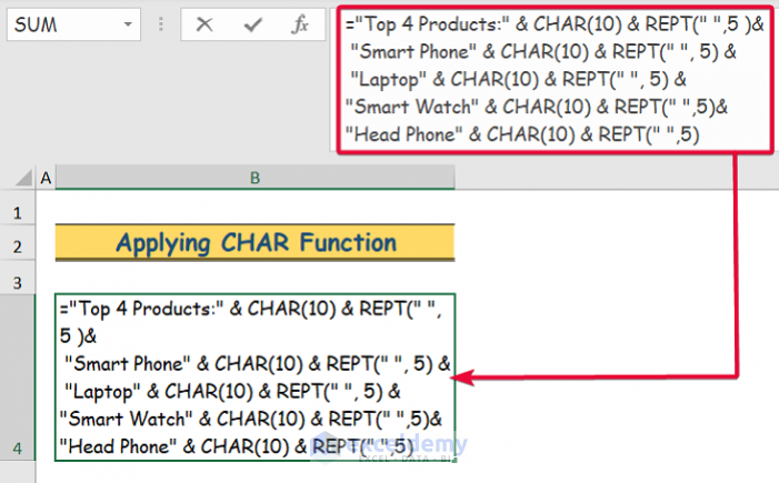
- Select the B4 cell.
- Copy the following formula,
="Top 4 Products:" & CHAR(10) & REPT(" ",5 )& "Smart Phone" & CHAR(10) & REPT(" ", 5) & "Laptop" & CHAR(10) & REPT(" ", 5) &"Smart Watch" & CHAR(10) & REPT(" ",5)&"Head Phone" & CHAR(10) & REPT(" ",5)- Hit Enter.
- Go to the Home tab.
- From the Alignment group, select Wrap Text.
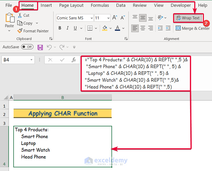
- This will insert a tab before your data and put it in a single cell.
Formula Break Down
- “Top 4 Products:” & CHAR(10) & REPT(” “,5 ): This is a repetitive formula. We will see this same connotation throughout the entire formula, which seems very long. The “Top 4 Products:” is the text that is added to the CHAR(10) function with the ampersand operator. CHAR(10) means “newline”. That means the cursor will go to a new line after the text. Finally, we concatenated the REPT(“ “, 5) notation with the CHAR(10) The REPT(“ “, 5) means the REPT or repeat function will repeat the space 5 times. That means the new line will have 5 spaces before the next text begins. These five spaces are equivalent to a tab in word documents.
Download Practice Workbook
Related Articles
- Add Blank Space Using Excel Formula
- How to Add Space between Rows in Excel
- How to Space Columns Evenly in Excel
- Space out Cells in Excel
- How to Space Rows Evenly in Excel
- Add Space between Numbers in Excel
- How to Add Space Between Text in Excel Cell
<< Go Back to Space in Excel | Text Formatting | Learn Excel
Get FREE Advanced Excel Exercises with Solutions!

In one cell a name and then a tab with date
Hello G,
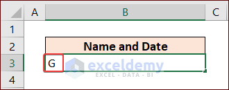
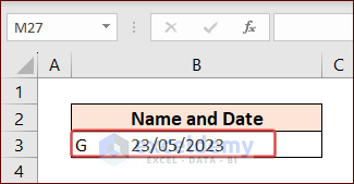
I think that you want to write a name, then some spaces, and then a date in one cell in Excel. Am I right? If that’s the matter, the solution is quite easy.
At first, select the cell (e.g. cell B3) and write your desired name. In this case, we wrote G.
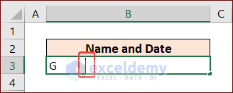
Then, press the SPACE button multiple times according to the space you need. Here, we gave 10 spaces to create an indentation.
Next, write the date like the following image.
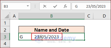
Finally, press the ENTER key. And the ultimate outcome is as follows.
Look, this is quite easy. But, if you want to mean something else, please write specifically. It’ll be helpful for us.
Thanks for your comment.
Regards,
SHAHRIAR ABRAR RAFID
Team ExcelDemy