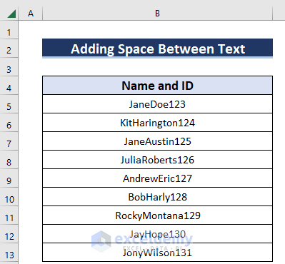
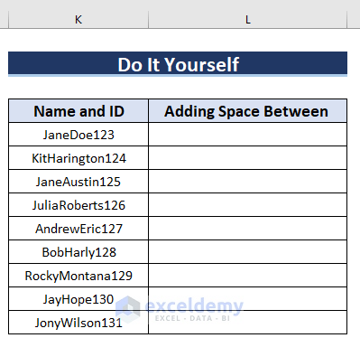
How to Add Space Between Text in a Cell in Excel (4 Easy Ways)

We imported Name and ID data into Excel as merged text. We want to make a proper structure of Name and ID.

How to Add Space Between Text in a Cell in Excel: 4 Easy Ways

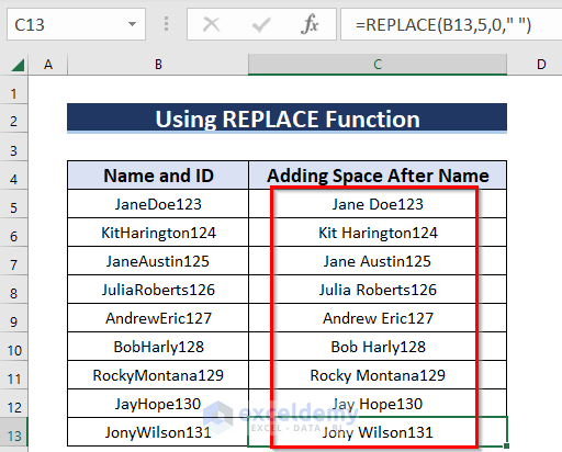
Method 1 – Using the REPLACE Function to Put a Space Between Text

The REPLACE function replaces specified parts of the text string with a newly assigned text string. Its syntax is:

REPLACE (old_text, start_num, num_chars, new_text)

old_text; refers to any reference cell you want the text to be replaced. start_num; declares from which number of character replacing will happen.
num_chars; defines how many characters will get replaced.
new_text; is the text that ultimately will be in the place of replaced characters.

Steps:

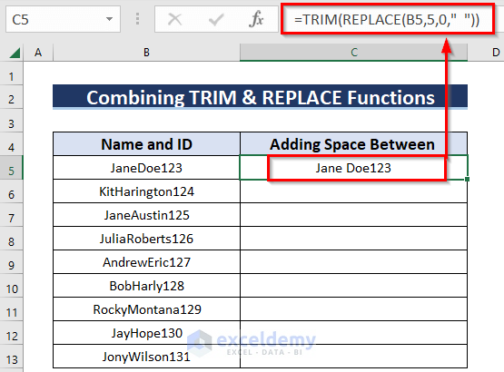
Use the following formula in cell C5.

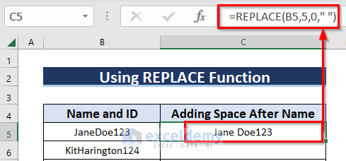
=REPLACE(B5,5,0," ")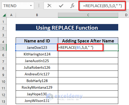

Formula Breakdown

B5 is the old_text reference. We have the text “JaneDoe123” in cell B5. We want the text as “Jane Doe123”.
We’ll put a space at the starting character start_num “5” (i.e after Jane).
We do not want any character to replace, so num_chars is “0”.
The new_text will be the space.

Press Enter.

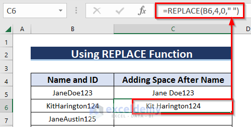
For the C6 cell, use the following formula (“Kit” has “3” letters, including the space, it will be “4”):

=REPLACE(B6,4,0," ")

Press Enter.

Repeat this process for other cells, changing the value of the second argument to match the location after the first name.

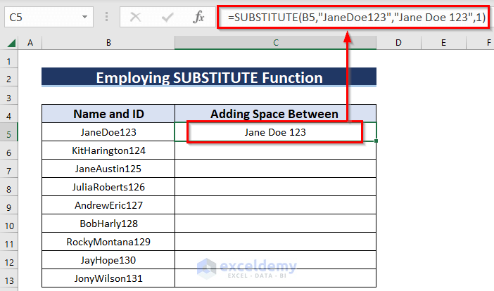
Method 2 – Applying the SUBSTITUTE Function to Add a Space Between Text

The syntax of the SUBSTITUTE function is:

SUBSTITUTE(text, old_text, new_text, [instance_num])

text; directs to any reference cell you want the text to substitute.
old_text; defines the text in the reference cell you want to substitute.
new_text; declares the text you the old_text to substitute with.
[instance_num]; defines the number of occurrences in old_text you want to substitute.

Steps:

Insert this formula in C5.

=SUBSTITUTE(B5,"JaneDoe123","Jane Doe 123",1)

Hit Enter.

Formula Breakdown

In the formula, B5 is the old_text reference.
Here, we have the text “JaneDoe123” in cell B5. But we want the text as “Jane Doe 123”.
Furthermore, the [instance_num] is “1”, as we have only one instance in the reference cell B5.

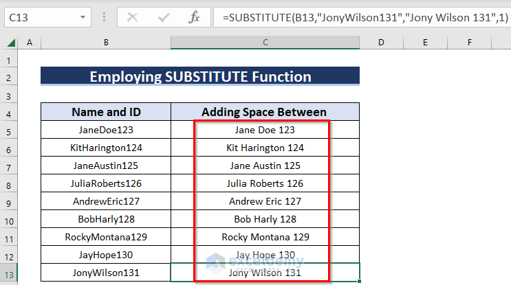
Here’s the formula for C6:

=SUBSTITUTE(B6,"KitHarington124","Kit Harington 124",1)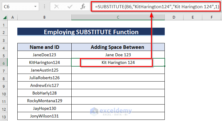

Change the formula for each cell accordingly.

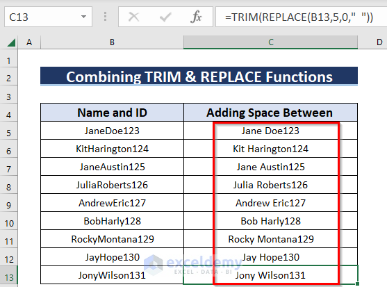
Method 3 – Merging TRIM and REPLACE Functions in Excel

Steps:

Insert the following formula in C5:

=TRIM(REPLACE(B5,5,0," "))

Here, the REPLACE function part in the formula works as in Method 1. TRIM removes the excess spaces before and after the string.

Press Enter.

Here’s the corresponding formula for C6.

=TRIM(REPLACE(B6,4,0," "))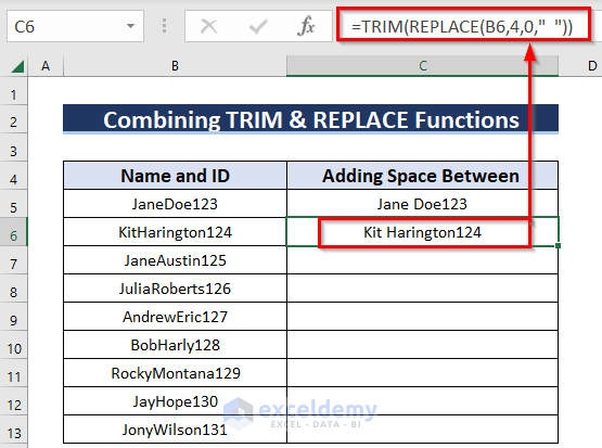

Repeat the process for other cells, changing the values as needed.

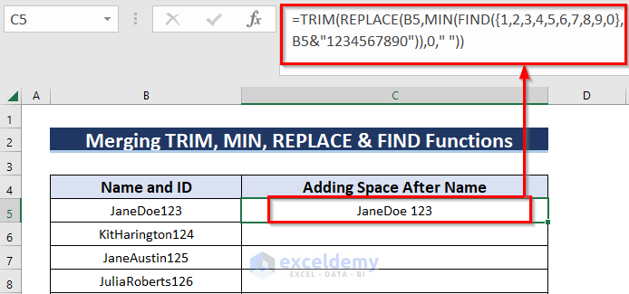
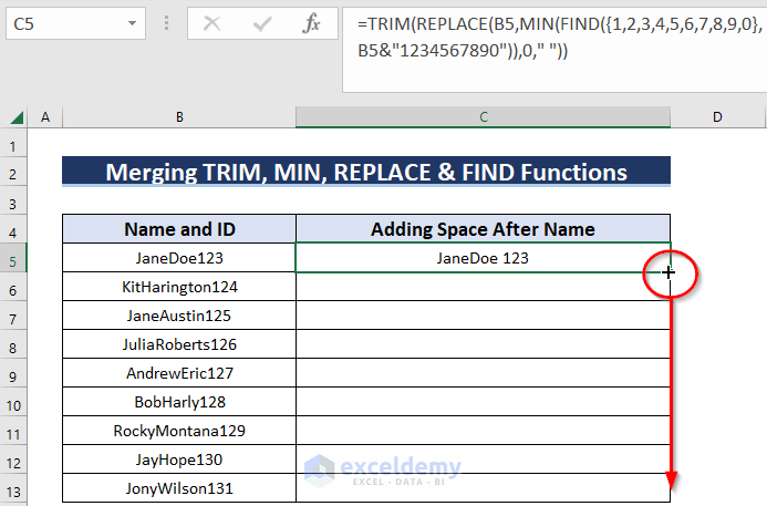
Method 4 – Combining TRIM, REPLACE, MIN and FIND Functions

We’ll put a space between the Name and ID in our dataset.

Steps:

Select C5 and enter the following formula.

=TRIM(REPLACE(B5,MIN(FIND({1,2,3,4,5,6,7,8,9,0},B5&"1234567890")),0," "))

Press Enter.

Formula Breakdown

B5&”1234567890″—> here the Ampersand operator (&) will join them.
- Output: “JaneDoe1231234567890”.
FIND({1,2,3,4,5,6,7,8,9,0},”JaneDoe1231234567890″)—> the FIND function will find the position (counting from “J”) of given numbers within the certain text.
- Output: {8,9,10,14,15,16,17,18,19,20}.
MIN({8,9,10,14,15,16,17,18,19,20})—> the MIN function will give the lowest number from the given array.
- Output: 8.
REPLACE(B5,8,0,” “)—> here the REPLACE function will introduce a space after the 7th number character of the B5 cell.
- Output: “JaneDoe 123”.
The TRIM function will remove all the extra spaces except a single space from the above text.

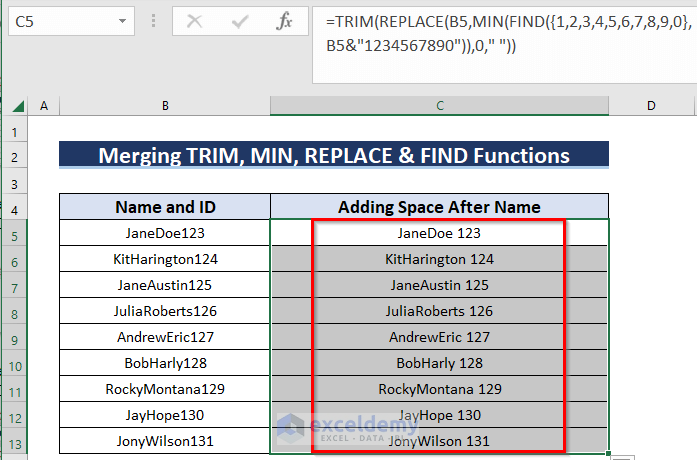
Drag the Fill Handle icon down to paste the formula to the other cells of the column.

Here’s the result.

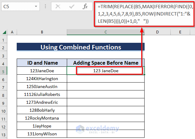
How to Include a Space Between Numbers and Text in Excel

Suppose we have the reverse, where the ID is before the name.

Steps:

Use the following formula in C5.

=TRIM(REPLACE(B5,MAX(IFERROR(FIND({0,1,2,3,4,5,6,7,8,9},B5,ROW(INDIRECT("1:"&LEN(B5)))),0))+1,0," "))

Hit Enter.

Formula Breakdown

LEN(B5)—> gives 10.
INDIRECT(“1:”&10)—> returns the array of 1:10.
The ROW function will give the row numbers of the above array.
- Output: {1;2;3;4;5;6;7;8;9;10}.
The FIND function will find the position of given numbers within the B5 cell.
The IFERROR function will convert all the error values into 0.
The MAX function will give the maximum number from the given array.
- Output: 4.
REPLACE(B5,4,0,” “)—> here the REPLACE function will introduce a space after the 3rd number character of the B5 cell.
- Output: “123 JaneDoe”.
The TRIM function will remove all the extra spaces except a single space from the above text.

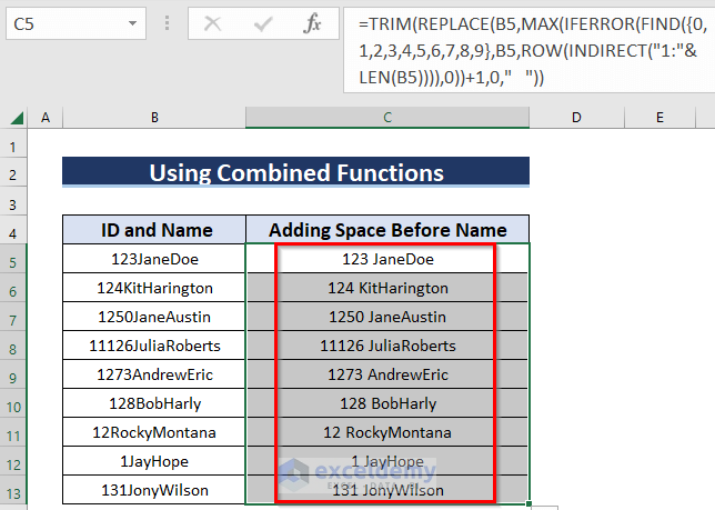
Drag the Fill Handle icon down to fill the column.

Practice Section

You can practice the explained methods in our download file.

Download the Practice Workbook

Adding Space Between Text.xlsx

<< Go Back to Space in Excel | Text Formatting | Learn Excel

Get FREE Advanced Excel Exercises with Solutions!

Function InsertSpacesAroundNumbers(inputText As String) As String Dim outputText As String Dim i As Integer Dim num As String Dim insideNumericSequence As Boolean outputText = "" insideNumericSequence = False For i = 1 To Len(inputText) num = Mid(inputText, i, 1) If IsNumeric(num) Then If Not insideNumericSequence Then outputText = outputText & " " insideNumericSequence = True End If outputText = outputText & num Else If insideNumericSequence Then outputText = outputText & " " insideNumericSequence = False End If outputText = outputText & num End If Next i outputText = Trim(outputText) Do While InStr(outputText, " ") > 0 outputText = Replace(outputText, " ", " ") Loop outputText = Trim(outputText) InsertSpacesAroundNumbers = outputText End Function

4 Comments

Emily Nov 1, 2022 at 4:02 AM

I used Method 3 and it worked great, however, how do I get rid of the column that is incorrect (without the edits/added space). Since they are dependent on each other, an error pops up when trying to remove the column that needed editing in the first place.
Shahriar Nov 3, 2022 at 11:07 AM

Hello Emily,
It is very motivating for us when someone benefits from using our method. Now getting back to your query. You can use a simple copy-paste feature to overcome this issue. Let’s see the process below for a better understanding.
• Firstly, select cells in the C5:C13 range.
• Then, press the CTRL key followed by the C key on the keyboard.

This command copies the whole range.
• After that, right-click on cell E5.
• In the context menu, select Values (V) in the Paste Options.

You can see the data pasted in the new place.

• Additionally, select cells in the B5:B13 range and C4:C13 range also.
• Therefore, delete them using the Delete button.

• At this time, press CTRL+C to copy the cells in the D5:D13 range.

• Henceforth, go to cell B5 and paste them by pressing CTRL+V.

Finally, you get the desired result.
LILY Nov 16, 2023 at 6:00 PM

Hello, I used the formula from the last section “How to Include Space Between Numbers and Text in Excel” but for some of the rows it inserts me spaces also between the numbers.
For example, for the text “VIA MARIO CARBONI 33F” the result is “VIA MARIO CARBONI 3 3F”. But for “VIA MARIO CARBONI 32F” the result is correct “VIA MARIO CARBONI 32F”.
Could you please help me better understand why for some texts the space is not displayed properly and how can I fix it?
Thank you
- Reply
  Sishir Roy Nov 20, 2023 at 12:44 PM
  Hello LILY,
  The formula used in the section “How to Include Space Between Numbers and Text in Excel” is a complex formula designed to insert a space after the rightmost numeric sequence in the text in a cell and then trim any extra spaces. It does not insert a space before the numeric sequence and only inserts a space after the rightmost numeric sequence. For example, you can see the image below.
  
  The issue you are facing might be due to certain functions not working correctly in your Excel version. Consider using the latest version to avoid these problems.
  However, the formula in the provided section does not insert space before the numeric sequence, making it less versatile. If you wish to insert a space between text and numbers regardless of the order of the numeric sequence, I can provide you with a VBA code to address this. If you want to insert a space before and after each numeric sequence without spaces between individual digits, you can use the following VBA function:
```
Function InsertSpacesAroundNumbers(inputText As String) As String
    Dim outputText As String
    Dim i As Integer
    Dim num As String
    Dim insideNumericSequence As Boolean

    outputText = ""
    insideNumericSequence = False

    For i = 1 To Len(inputText)
        num = Mid(inputText, i, 1)

        If IsNumeric(num) Then
            If Not insideNumericSequence Then
                outputText = outputText & " "
                insideNumericSequence = True
            End If
            outputText = outputText & num
        Else
            If insideNumericSequence Then
                outputText = outputText & " "
                insideNumericSequence = False
            End If
            outputText = outputText & num
        End If
    Next i

    outputText = Trim(outputText)

    Do While InStr(outputText, "  ") > 0
        outputText = Replace(outputText, "  ", " ")
    Loop

    outputText = Trim(outputText)
    InsertSpacesAroundNumbers = outputText
End Function
```
  To use this, open the VBA launcher by pressing the Alt+F11 button on your keyboard.
  Click on the Insert button and choose the Module option.
  In the Module section, paste the provided VBA code.
  
  After that, go back to your Excel file, and type the function name ‘=InsertSpacesAroundNumbers‘. You will find the function name in the function list. Put the cell reference in the function argument and press Enter.
  
  As a result, it will insert a space before and after each numeric sequence without inserting spaces between individual digits.
  
  Regards,
  Sishir Roy

How to Add Space Between Text in a Cell in Excel (4 Easy Ways)

How to Add Space Between Text in a Cell in Excel: 4 Easy Ways

Method 1 – Using the REPLACE Function to Put a Space Between Text

Method 2 – Applying the SUBSTITUTE Function to Add a Space Between Text

Method 3 – Merging TRIM and REPLACE Functions in Excel

Method 4 – Combining TRIM, REPLACE, MIN and FIND Functions

How to Include a Space Between Numbers and Text in Excel

Practice Section

Related Articles

Leave a reply Cancel reply