How to Use the SUMPRODUCT with INDEX and MATCH Functions in Excel

Introduction to the Functions: SUMPRODUCT, INDEX and MATCH (with Examples)

Before delving into how these three powerful functions work together, let’s introduce each function and understand their individual processes:

1. SUMPRODUCT Function

• Syntax: =SUMPRODUCT(array1,[array2],[array3],…)

• Function: Returns the sum of the products of corresponding ranges or arrays.

• Example: Suppose we have a dataset with a list of computer devices from different brands, along with their selling prices for six months in a computer shop. We want to calculate the total selling price of desktops for January only.

Steps:

• In cell F18, enter the following formula:

• Here, C5:C14 represents the Device Category column, F16 is the selected Device, and D5:D14 contains the Jan sales data.
• Press ENTER to see the total selling price of all desktops for January.

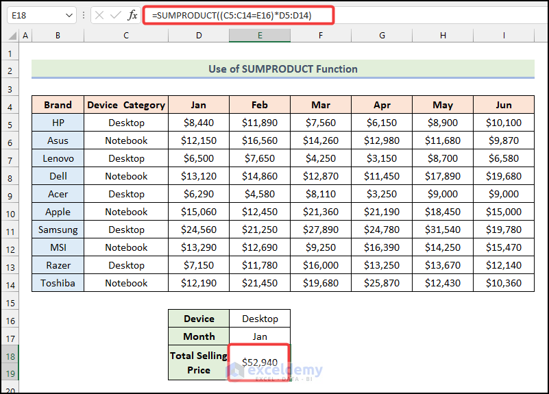
Inside the SUMPRODUCT function, there is only one array. Here, C5:C14=F16 means we’re instructing the function to match criteria from cell F16 in the range of cells C5:C14. By adding another range of cells D5:D14 with an Asterisk(*) before, we’re telling the function to sum up all the values from that range under the given criteria.

2. INDEX Function

• Syntax: =INDEX(array, row_num, [column_num])

or,

=INDEX(reference, row_num, [column_num], [area_num])

• Function: Returns the value of a cell at the intersection of a specific row and column within a given range.

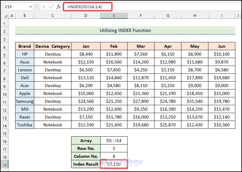
• Example: Let’s find the value at the intersection of the 3rd row and 4th column from an array of selling prices.

Steps:

• In cell F19, type:

• Press ENTER to get the result. This corresponds to the selling price of Lenovo desktops in April.

Since the 4th column in the array represents the selling prices of all devices for April & the 3rd row represents the Lenovo Desktop Category, at their intersection in the array, we’ll find the selling price of Lenovo desktop in April.

3. MATCH Function

• Syntax: =MATCH(lookup_value, lookup_array, [match_type])

• Function: Returns the relative position of an item in an array that matches a specified value in a specified order.

• Example: To determine the position of the month of June from the month headers

Steps:

• In cell F17, use the formula:

• Press ENTER to find that the column position for June is 6 in the month headers.

If you change the name of the month in cell F17, you’ll see the related column position of another month selected.

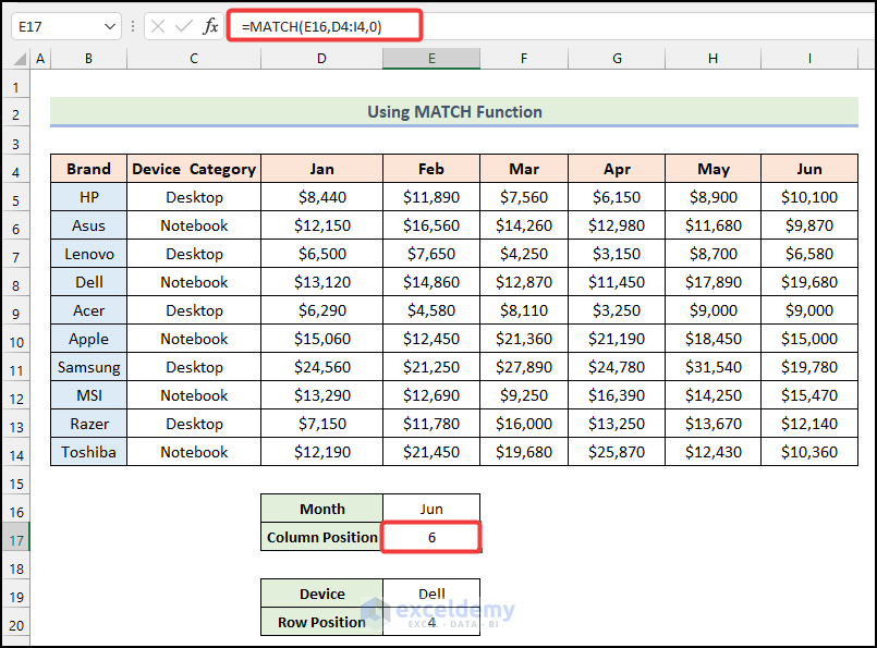
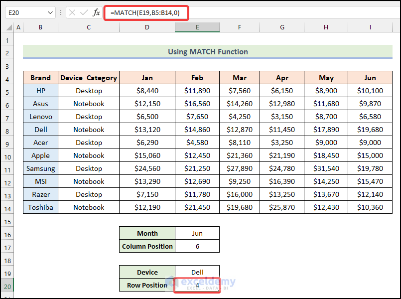
Similarly, if you want to know the row position of the brand “Dell” from the brand names in Column B, use the formula in cell F20:

Changing the brand name in cell F19 will give you the related row position for that brand within the selected range of cells.

Using INDEX and MATCH Functions Together in Excel

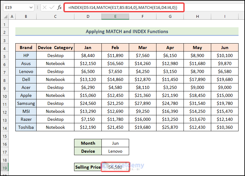
Scenario: Finding the Total Selling Price of Lenovo Brand in June

Suppose we have a dataset with information about computer devices, including their brands and selling prices for different months. We want to determine the total selling price of the Lenovo brand in June.

Steps:

• In cell E19, type the following formula:

• • Explanation:
    • E17 refers to the selected device (Lenovo).
    • The range B5:B14 contains the brand names.
    • E16 represents the selected month (June).

• Press ENTER to get the total selling price instantly.

If you change the month or device name in E16 or E17, the result in E19 will update accordingly.

Using SUMPRODUCT with INDEX and MATCH Functions

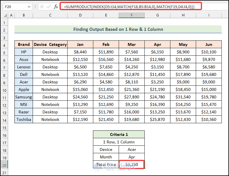
Criteria 1: Finding Output Based on 1 Row & 1 Column 

Based on our 1st criterion, we want to know the total selling price of the Acer brand in the month of April.

Steps:

• In cell F20, use the formula:

• • Explanation:
    • F18 represents the selected device (Acer).
    • F19 corresponds to the month (April).
    • The result is $3,250.

• After that, press ENTER & the return value will be $3,250.

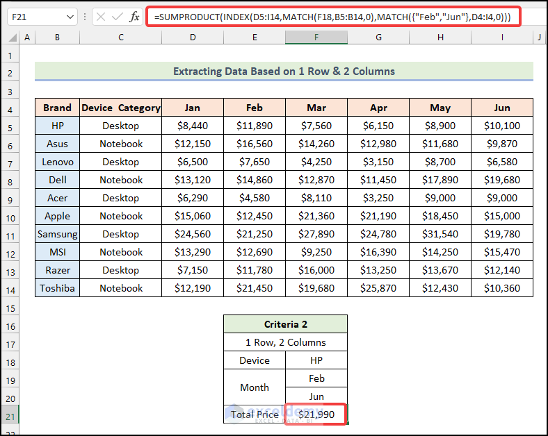
Criteria 2: Extracting Data Based on 1 Row & 2 Columns 

Now we want to know the total selling price of HP devices in the months of February as well as June.

Steps:

• In cell F21, type:

• • Explanation:
    • The curly brackets define the months (February and June).
    • The result is $21,990.

• After pressing ENTER, you’ll find the resultant value as $21,990.

Criteria 3: Determining Values Based on 1 Row & All Columns 

In this part, we’ll deal with all columns with 1 fixed row. So, we can find the total selling price of Lenovo devices in all months under our criteria here.

Steps:

• In cell F20, use:

• • Explanation:
    • The 0 argument in the second MATCH function considers all columns.
    • The result is $36,830.

• Press ENTER & you’ll find the total selling price as $36,830.

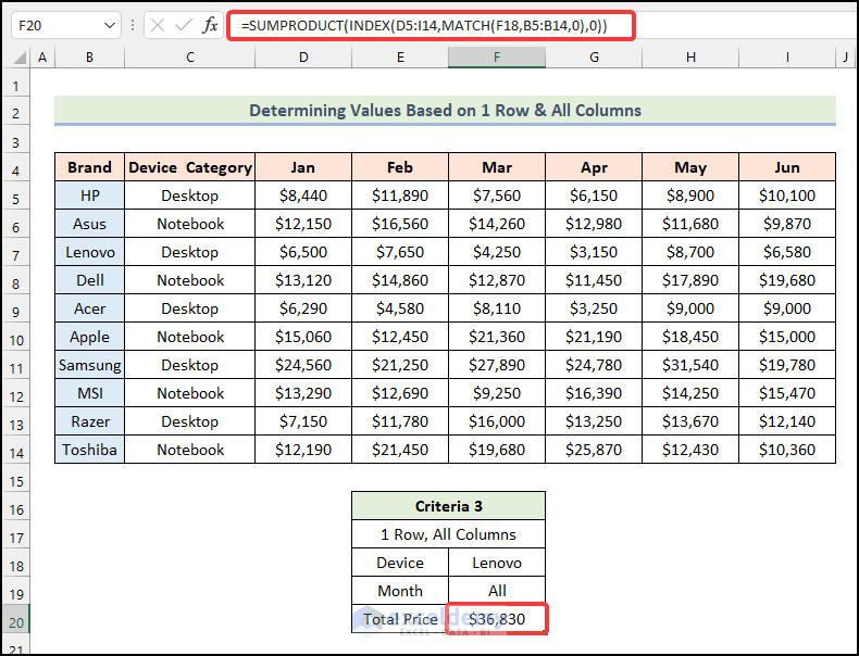
In this function, to add criteria for considering all months or all columns, we have to type 0 as the argument- column_pos inside the MATCH function.

Criteria 4: Calculating Sum Based on 2 Rows & 1 Column 

In this section under 2 rows & 1 column criteria, we’ll find out the total selling price of HP & Lenovo devices in the month of June.

Steps:

• In cell F21, the formula will be under the given criteria:

• • • Cell F20 represents the selected Month.

• After pressing ENTER, we’ll find the return value as $16,680.

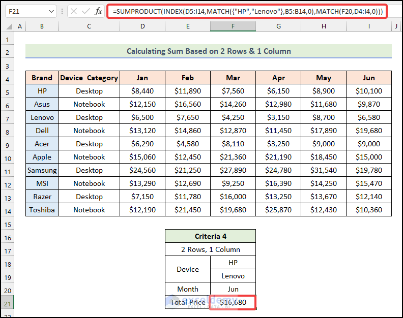
Here inside the first MATCH function, we have to input HP & Lenovo inside an array by enclosing them with curly brackets.

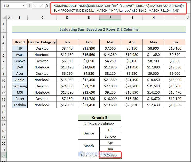
Criteria 5: Evaluating Sum Based on 2 Rows & 2 Columns 

Now we’ll consider 2 rows & 2 columns to extract the total selling prices of HP & Lenovo devices for two particular months- April & June.

Steps:

• Type the following formula in cell F22:

• • Explanation:
    • We’re using two SUMPRODUCT functions, one for April and one for June.
    • The curly brackets define the months.
    • Output: $25,980

We incorporated two SUMPRODUCT functions by adding a Plus(+) between them for two different months.

• Press ENTER & you’ll see the output as $25,980.

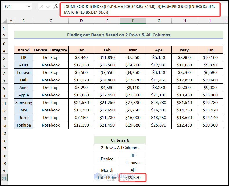
Criteria 6: Finding out Result Based on 2 Rows & All Columns 

In this part, let’s deal with 2 rows & all columns. So, we’ll find out the total selling prices for HP & Lenovo devices in all months.

Steps:

• Our formula will be in cell F21:

• • Explanation:
    • We’re using two SUMPRODUCT functions, one for each device (HP and Lenovo) across all months.
    • Output: $89,870

Like in the previous method, we incorporate two SUMPRODUCT functions by adding a Plus(+) between them for 2 different Devices for all months.

• Press ENTER & we’ll find the resultant value as $89,870.

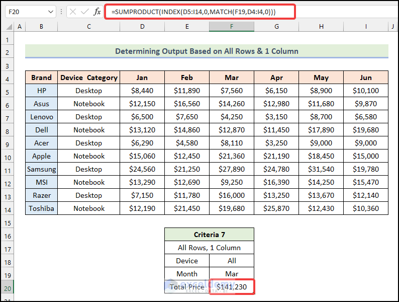
Criteria 7: Determining Output Based on All Rows & 1 Column 

Under this criterion, we can now extract the total selling prices of all Devices for a single month (March).

Steps:

• Insert the formula in cell F20:

• Press ENTER. The return value will be $141,230.

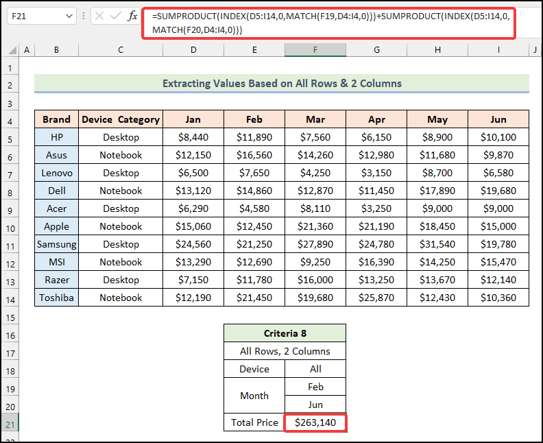
Criteria 8: Extracting Values Based on All Rows & 2 Columns 

In this part, we’ll determine the total selling price of all devices for two months- February & June.

Steps:

• In cell F21, we have to type:

• • Explanation:
    • We’re using two SUMPRODUCT functions, one for February and one for June.
    • Output: $263,140

Here, we are applying two SUMPRODUCT functions by adding a Plus(+) between them for 2 different Months for all Devices.

• After pressing ENTER, the total selling price will appear as $263,140.

Criteria 9: Finding Result Based on All Rows & All Columns 

We’ll now find out the total selling price of all Devices for all months in the table.

Steps:

• In cell F20, you have to type:

• • Explanation:
    • We’re considering all columns and rows.
    • Output: $808,090

• Press ENTER & you’ll get the resultant value as $808,090.

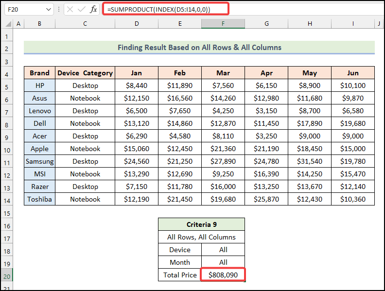
You don’t need to use MATCH functions here as we’re defining all columns & row positions by typing 0’s inside the INDEX function.

Criteria 10: Calculating Sum Based on Distinct Pairs 

In our final criterion, we’ll find out the total selling prices of HP devices for April along with Lenovo devices for June together.

Steps:

• Under this criterion, our formula in cell F22 will be:

• • Explanation:
    • The first MATCH function returns the row numbers for “HP” and “Lenovo” devices.
      • Output: {1, 3}
    • The second MATCH function returns the column numbers for April and June.
      • Output: {4, 6}
    • The INDEX function retrieves the selling prices based on the intersections of rows and columns.
    • Finally, the SUMPRODUCT function adds up the selling prices.
      • Output: $12,730

• Now press ENTER & you’ll see the result as $12,730.

When using distinct pairs in this combined function, ensure that the device and month names are correctly placed inside the arrays corresponding to row and column positions. The order of device and month names matters.

SUMPRODUCT vs INDEX-MATCH

• SUMPRODUCT Function:
  • Returns the sum of the products of selected arrays.
  • Can be used as an alternative to array formulas.
  • Useful for various analyses and comparisons with multiple criteria in Excel.
• INDEX-MATCH Combination:
  • Efficient alternative to lookup functions in Excel.
  • Allows searching for specific values within a specified dataset.
  • Combining SUMIFS with INDEX-MATCH can handle conditional sums for multiple criteria.

Download Practice Workbook

You can download the practice workbook from here:

<< Go Back to INDEX MATCH | Formula List | Learn Excel