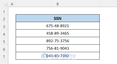
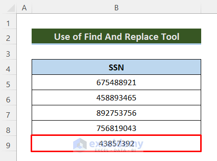
We’ll use the following dataset, which contains some random SSNs.
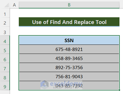
Method 1 – Apply the Find and Replace Tool to Erase Dashes from SSNs in Excel
Steps:
- Select the data range.
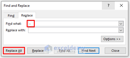
- Press Ctrl + H to open the Find and Replace tool.
- Put a hyphen(-) in the Find what: box and keep the Replace with: box empty.
- Press the Replace All button.
The Find and Replace tool has removed all the dashes from the SSNs. A pop-up message box shows how many replacements were made.
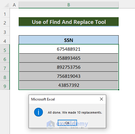
However, the zero (0) digits at the front are gone, too.
Read More: How to Remove Dashes in Excel
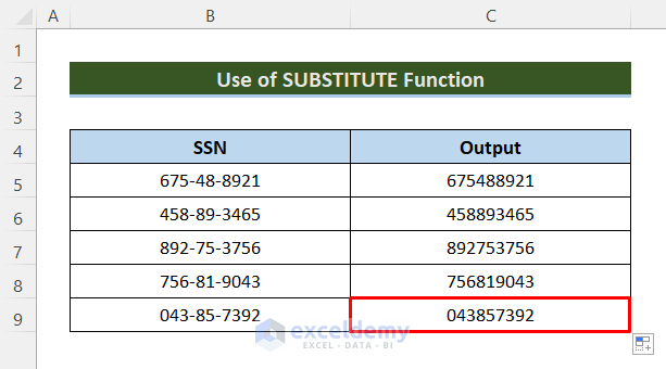
Method 2 – Use the SUBSTITUTE Function to Remove Dashes from SSNs in Excel
Steps:
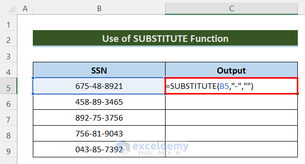
- Activate Cell C5 by pressing it.
- Insert the following formula in it:
=SUBSTITUTE(B5,"-","")- Hit the Enter button to get the output.
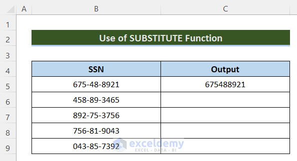
The output without dashes is:
- Drag down the Fill Handle icon to copy the formula and remove dashes from other SSNs.
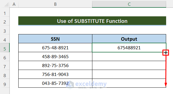
Here are our final results.
Read More: How to Remove Dashes from Phone Number in Excel
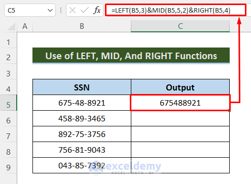
Method 3 – Combine LEFT, MID, and RIGHT Functions in Excel to Delete Dashes from SSNs
- In Cell C5, insert the following formula-
=LEFT(B5,3)&MID(B5,5,2)&RIGHT(B5,4)- Press the Enter button to get the result.
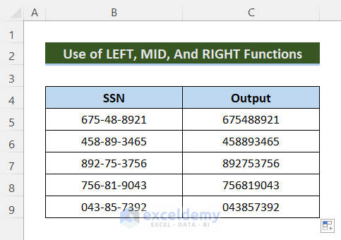
- To copy the formula for the other cells, drag the Fill Handle icon down.
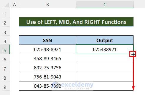
Soon after you will get all the output including zero at the beginning.
⏬ Formula Breakdown:
➥ LEFT(B5,3)
The LEFT function will keep the first three digits of the number in Cell B5. It will return:
“675”
➥ MID(B5,5,2)
Then the MID function will keep the two digits starting from the 5th digit of the number in Cell B5. The output is:
“48”
➥ RIGHT(B5,4)
Later, the RIGHT function will return the last 4 digits of the number in Cell B5 that will return:
“8921”
➥ LEFT(B5,3)&MID(B5,5,2)&RIGHT(B5,4)
And finally, those three previous outputs will be combined using &, as a result, the final output will return:
“675488921”
Read More: How to Remove Non-Alphanumeric Characters in Excel
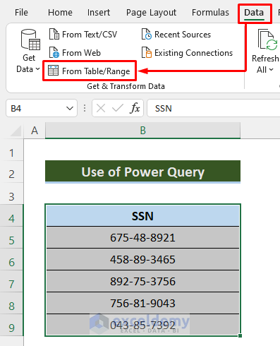
Method 4 – Use the Power Query Tool to Remove Dashes from SSNs
Steps:
- Select the range of cells B4:B9, including the header.
- Go to Data and select From Table/Range.
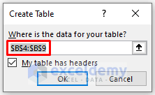
- Check the My table has headers option.
- Press OK.
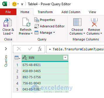
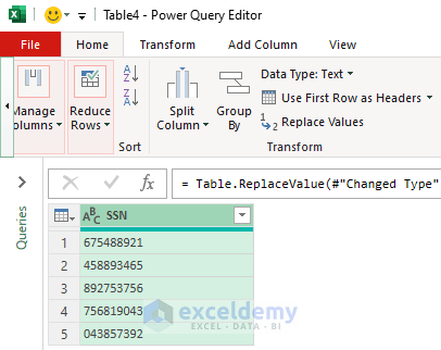
The Power Query Editor window will appear.
Our dataset will look like the following image after the Power Query Editor opens.
- Go to Home and select Replace Values.
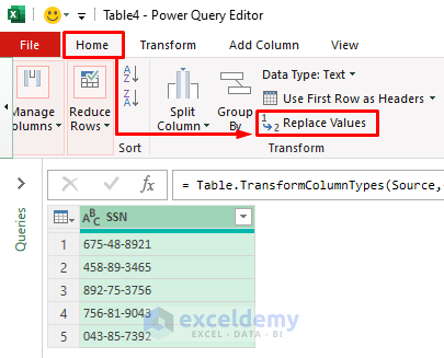
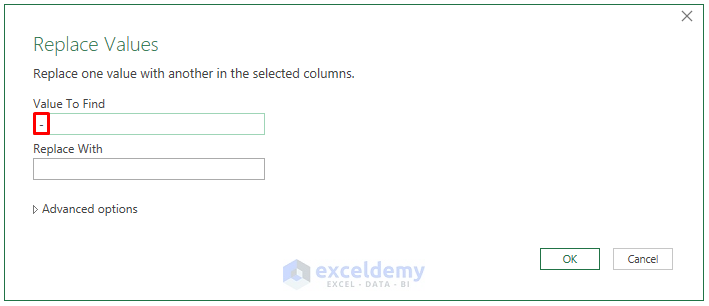
A dialog box named Replace Values will appear.
- Type a hyphen(-) in the Value to Find box and keep the Replace With box empty.
- Press OK.
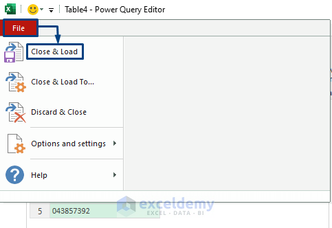
Power Query has deleted all the dashes.
- In the Power Query Editor window, click File and choose Close & Load.
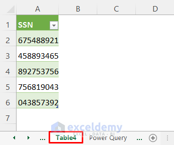
Here’s the new worksheet with the output from Power Query.
Download the Practice Workbook
Related Articles
- How to Remove Parentheses in Excel
- How to Remove Semicolon in Excel
- How to Remove Apostrophe in Excel
- How to Remove Asterisk in Excel
- How to Remove Non-Printable Characters in Excel
<< Go Back To Remove Specific Characters in Excel | Excel Remove Characters | Data Cleaning in Excel | Learn Excel
Get FREE Advanced Excel Exercises with Solutions!
