In this article, we will demonstrate 4 easy methods to remove parentheses in Excel.
What Are Parentheses in Excel?
In general, Parentheses are a pair of characters or symbols that group elements together, which have different expressions in different contexts. Common examples include (), {} and {}. In Excel, values inside parentheses are evaluated first, before other operations in a formula.
There are 2 scenarios involving parentheses in calculation in Excel:
- In the case of more than one parenthesis in a formula, the calculation is done from left to right.
- On the other hand, when there are multiple parentheses inside one another, they will be calculated in an inside-out process. So, the innermost formula or value is evaluated first and the outermost last.
How to Remove Parentheses in Excel: 4 Easy Ways
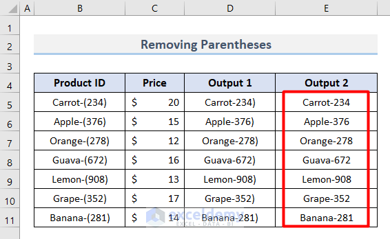
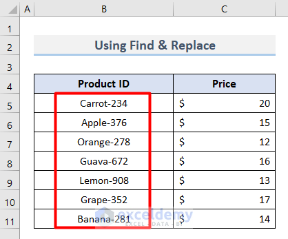
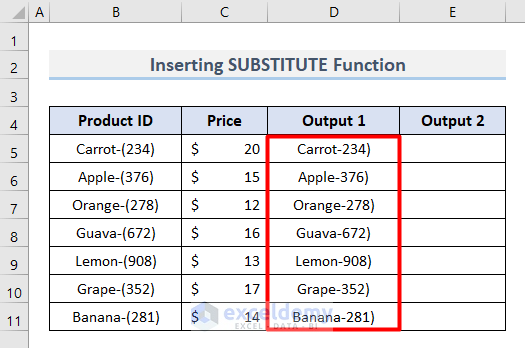
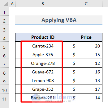
We’ll use the dataset below to illustrate our methods. There are numbers within parentheses in every Product ID. The numbers denote the product codes, whereas the parentheses are redundant.
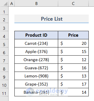
We’ll remove the parentheses using the methods below.
Method 1 – Using Find & Replace to Remove Parentheses
In this first method, we will use the Find & Replace command to remove the parentheses one at a time.
- Select the range B5:B11.
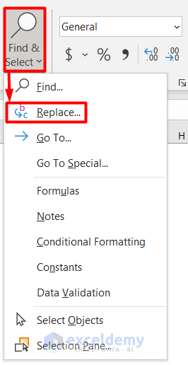
- Select Find & Select from the Home tab
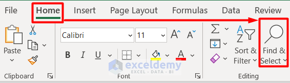
- In the drop-down menu, choose Replace.
The Find & Replace dialogue box opens. It can also be opened with the keyboard shortcut Ctrl + H.
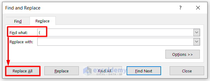
- Now, type “(“ in the Find what box and keep the Replace with box empty.
- Click Replace All to remove the opening bracket.
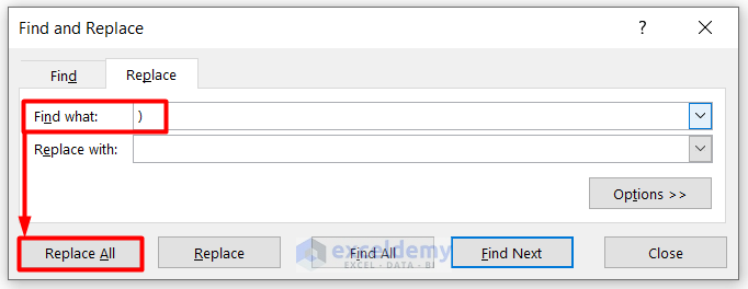
- Now type “)“ in the Find what box and keep the Replace with box empty.
- Click Replace All again.
The parentheses are removed completely.

Read More: How to Remove Non-Alphanumeric Characters in Excel
Method 2 – Using the SUBSTITUTE Function to Delete Parentheses in Excel
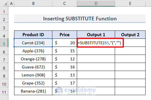
The SUBSTITUTE function finds text in a cell and replaces it with different text. First, we’ll remove the opening parenthesis in Column Output1, and then the closing parenthesis in Column Output2.
Steps:
- Select Cell D5 and enter the formula below:
=SUBSTITUTE(B5,"(","")- Press Enter.
- Drag the Fill Handle icon down to copy the formula to the cells below.
The opening parentheses are gone.
- In Cell E5, enter the following formula:
=SUBSTITUTE(D5,")","")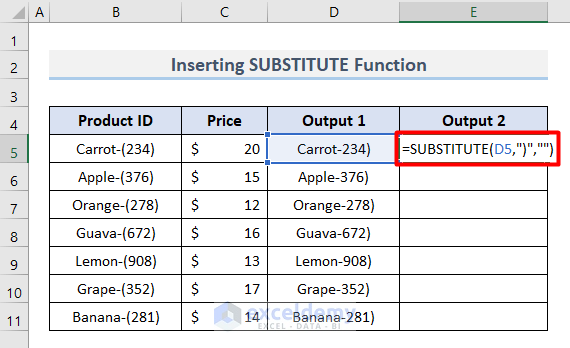
- Press Enter and drag the Fill Handle icon to copy the formula.
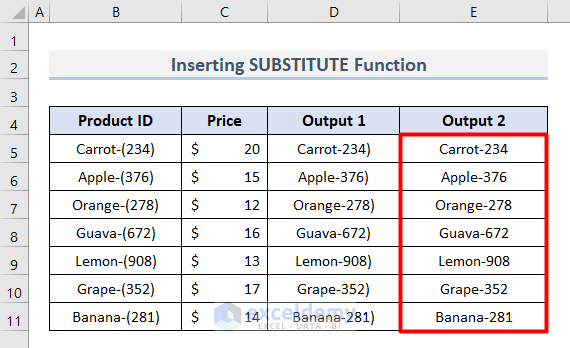
Both parentheses have now been removed
Method 3 – Using VBA Macros to Erase Parentheses in Excel
We can also remove all the parentheses using VBA code.
Steps:
- Right-click on the sheet title.
- Select View Code from the context menu .
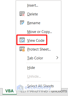
The VBA Module window will open up.
- Enter the following code in the window:
Option Explicit
Sub DelParentheses()
Cells.Select
Selection.Replace What:="(", Replacement:="", LookAt:=xlPart, _
SearchOrder:=xlByRows, MatchCase:=False, SearchFormat:=False, _
ReplaceFormat:=False
Selection.Replace What:=")", Replacement:="", LookAt:=xlPart, _
SearchOrder:=xlByRows, MatchCase:=False, SearchFormat:=False, _
ReplaceFormat:=False
End Sub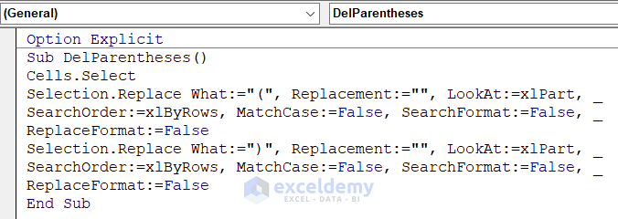
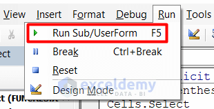
- Select the Run Sub from the Run tab to run the code.
All the parentheses are deleted from the selected range.
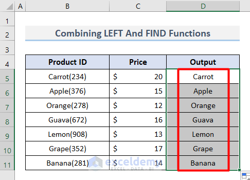
Method 4 – Combining the LEFT And FIND Functions to Remove Text with Parentheses in Excel
The LEFT function returns the first character or characters in a text string from the left based on the number of characters specified. The FIND function is used to find the position of a substring in a string. We can combine these functions to remove parentheses.
Steps:
- Enter the following formula in Cell D5:
=LEFT(B5,FIND("(",B5,1)-1)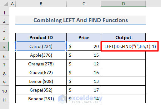
- Press Enter to return the output.
- Drag the Fill Handle icon down to copy the formula to the rest of the cells.
Formula Breakdown:
- FIND(“(“,B5,1)
Finds the position number of the opening parenthesis starting from the first position, and returns:
{7}
- LEFT(B5,FIND(“(“,B5,1)-1)
Keeps only 6 letters starting from the left, so 1 is subtracted from the output to remove the bracket. It returns:
{Carrot}
Download Practice Workbook
Related Articles
- How to Remove Dashes from Phone Number in Excel
- How to Remove Dashes from SSN in Excel
- How to Remove Semicolon in Excel
- How to Remove Apostrophe in Excel
- How to Remove Asterisk in Excel
- How to Remove Non-Printable Characters in Excel
- How to Remove Dashes in Excel
<< Go Back To Remove Specific Characters in Excel | Excel Remove Characters | Data Cleaning in Excel | Learn Excel
Get FREE Advanced Excel Exercises with Solutions!
