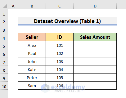
We have two sheets named Table 1 and Table 2. In the first sheet, we have a table that contains the seller’s info.
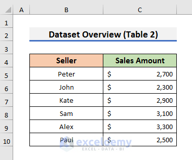
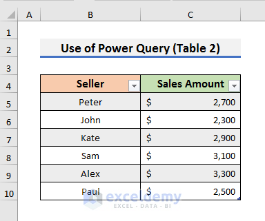
In the second sheet, we have another table that contains the sales amount. We will merge these two tables based on the Seller column. Here, the order of the sellers is not the same as in the first table.
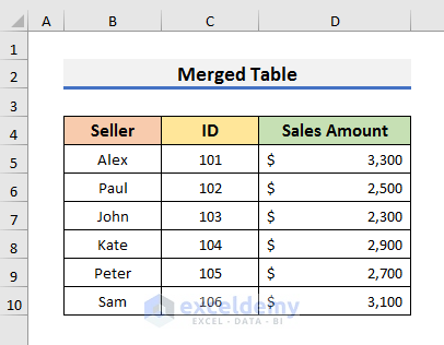
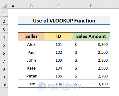
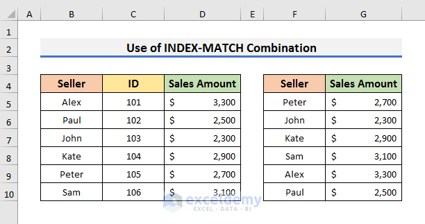
After merging, the merged table will look like the dataset below.
Method 1 – Merging Two Tables Based on One Column Using a Formula in Excel
Case 1.1 – Apply the VLOOKUP Function
STEPS:
- Go to the first table and select Cell D5.
- Use the formula below in Cell D5:
=VLOOKUP(B5:B10,'Table 2'!B5:C10,2,FALSE)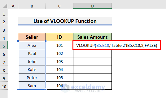
In this formula, we have four arguments inside the VLOOKUP function.
- Range B5:B10 is the lookup value. That means the formula will look for these values in Table 2.
- The second argument denotes the table array of the Table 2 sheet. After typing the first argument, you need to type a comma (,) and move to the sheet that contains the second table. Then, select the table array from there.
- The third argument denotes the second column of Table 2 and FALSE denotes the exact match.
- Press Ctrl + Shift + Enter to get the results.
Note: As VLOOKUP looks for the value in the leftmost column of a table, it can produce errors and return incorrect results. It is also unable to extract data from a column left to the lookup column.
Case 1.2 – Insert an INDEX-MATCH Formula Combination
The general form of the INDEX–MATCH can be written as:
=INDEX(return_range, MATCH(lookup_value, lookup_range,0))Steps:
- Select cell D5 and use the formula below:
=INDEX('Table 2'!$C$5:$C$10,MATCH('INDEX-MATCH'!$B5,'Table 2'!$B$5:$B$10,0))- Hit Enter to see the result.
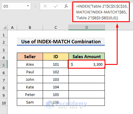
In this formula, we have merged two tables from the sheets named Table 2 and INDEX–MATCH.
- Table 2′!$C$5:$C$10: The return range. The sheet named Table 2 contains this range of the second table.
- ‘INDEX-MATCH’!$B5: The lookup value. The sheet named INDEX–MATCH contains this value.
- ‘Table 2’!$B$5:$B$10: The lookup range. The formula looks for the value of Cell B5 of the INDEX–MATCH sheet in the range B5:B10 of the Table 2 sheet.
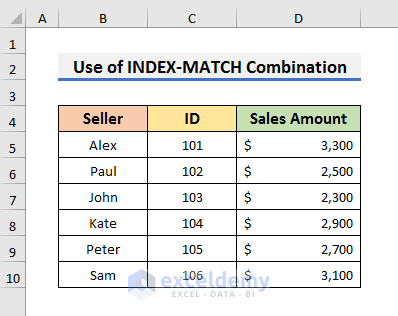
- Drag the Fill Handle down to merge two tables.
We can also use this formula to merge tables from the same sheet. You can see Table 1 and Table 2 on the same sheet.
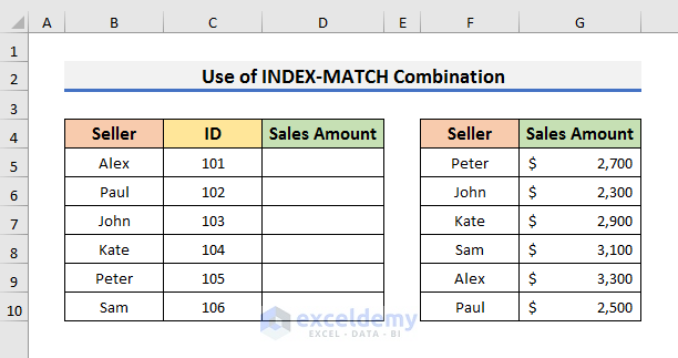
- Select cell D5 and use the formula below:
=INDEX($G$5:$G$10,MATCH($B5,$F$5:$F$10,0))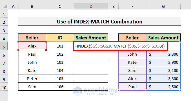
This formula works the same as the previous one we used in this method.
- Press Enter and drag the Fill Handle down.
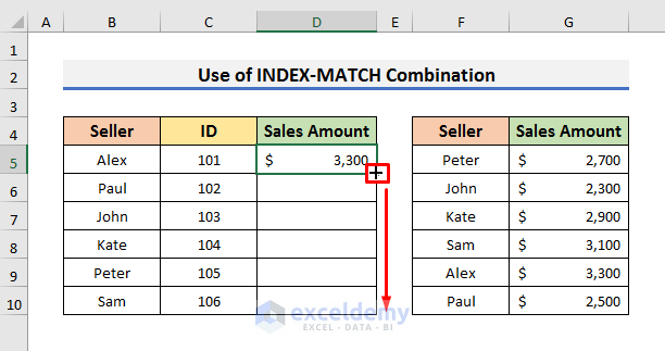
- You will see results like the picture below.
Read More: How to Merge Two Tables in Excel Using VLOOKUP
Method 2 – Use Excel Power Query to Join Two Tables Based on One Column
We will use the previous dataset, but there will be no Sales Amount column in Table 1. The name of the first table is Seller_Info.
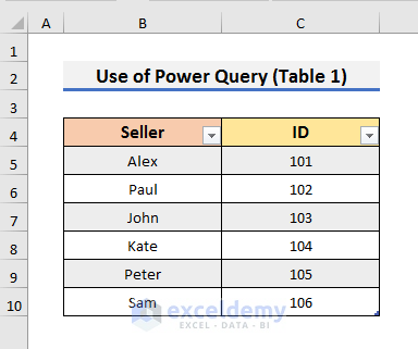
Table 2 will contain the sales amount. The name of the second table is Sales_Amount. Here, the Seller column is the common column between the two tables.
Steps:
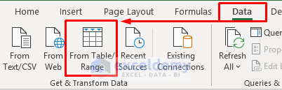
- Go to the sheet that contains the first table.
- Go to the Data tab and select From Table/Range. It will open the Power Query window.
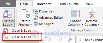
- In the Power Query window, go to the Home tab and click on the Close & Load icon. A drop-down menu will appear.
- Select Close & Load To. It will open the Import Data dialog box.
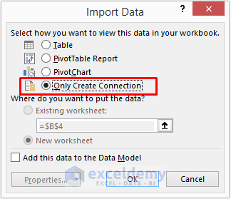
- In the Import Data box, select Only Create Connection and click OK to proceed.
- Repeat the above steps for the second table.
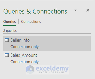
- You will see the tables in the Queries & Connections pan. Here, Seller_Info is the first table and Sales_Amount is the second table.
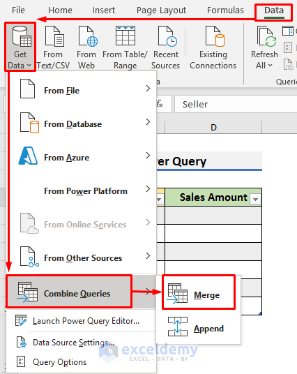
- Navigate to the Data tab and select Get Data. A drop-down menu will appear.
- Select Combine Queries and Merge. This will open the Merge window.
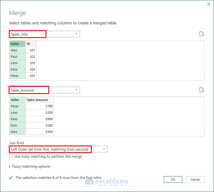
- In the Merge window, select the tables in the first two boxes.
- Select Left Outer (all from first, matching from second) in the Join Kind box.
- Select the Seller column in both tables.
- Click OK to proceed.
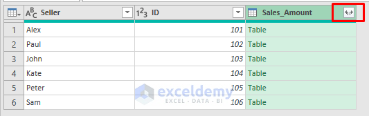
- You will see a merged table in the Power Query Editor. But the Sales Amount column doesn’t contain any value.
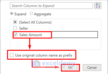
- Click on the Expand icon.
- A message box will appear.
- Unselect all columns from there and select Sales Amount again.
- Uncheck ‘Use original column name as prefix’.
- Click OK to proceed.
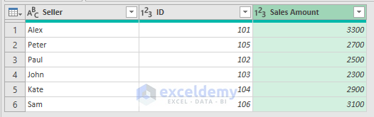
- You will see the merged table with values in the Sales Amount column.
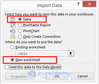
- To load the merged table, go to the Home tab of the Power Query window and click on the Close & Load icon.
- Select Close & Load To from the drop-down menu.

- Select Table and New worksheet in the Import Data box.
- Click OK.
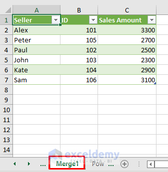
- You will see the merged table in a new sheet named Merge 1.
Method 3 – Merge Two Excel Tables Based on One Column with Copy and Paste Options
The tables have exactly the same values in the Seller column in the same order.
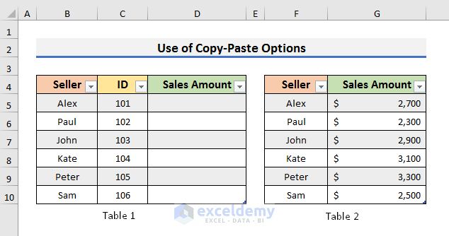
Steps:
- Select the range G5:G10 from the second table.
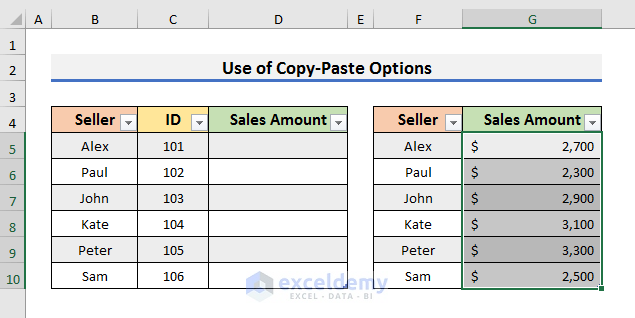
- Press Ctrl + C to copy.
- Select Cell D5.
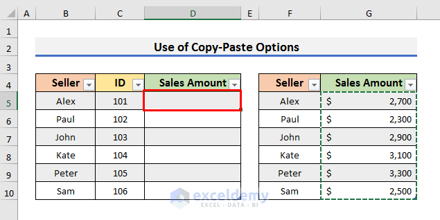
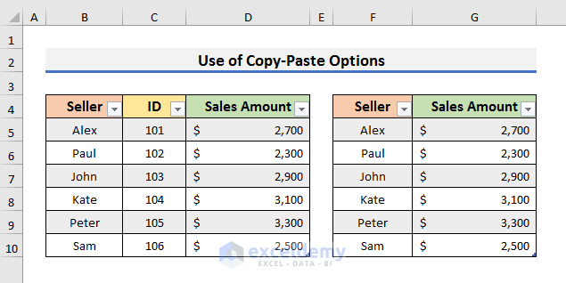
- Press Ctrl + V to paste the values of the second table into the first table.
Download the Practice Book
<< Go Back to Merge Tables in Excel | Merge in Excel | Learn Excel
Get FREE Advanced Excel Exercises with Solutions!
