How to Link Sheets in Excel with a Formula – 4 Methods

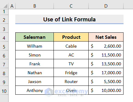
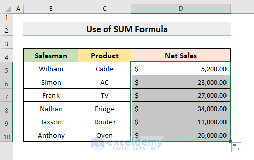
The following dataset showcases Salesman, Product, and Net Sales of a company.

Method 1 – Creating a Link Formula in Excel to Link Sheets

1.1 Same Workbook

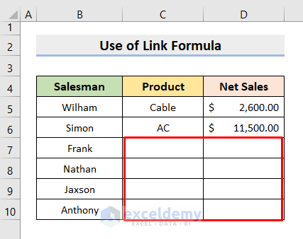
Data is missing in the link formula1 sheet and you want to insert data from the link formula2 sheet.

STEPS:

• Select C7 in link formula1 and enter the formula:

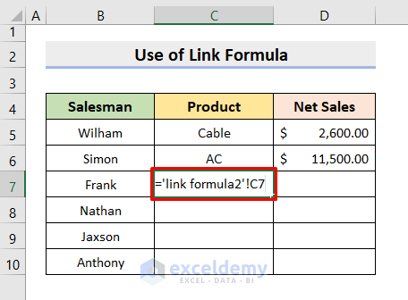
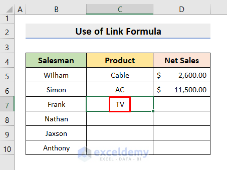
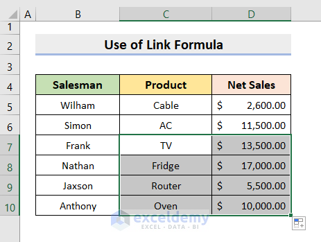
• Press Enter, and it’ll return the cell value in link formula2.

• Use the AutoFill .
• Check Fill Without Formatting in the AutoFill Options.

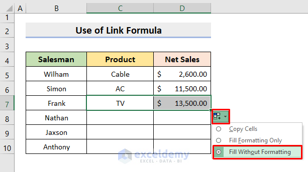
• Use the AutoFill  to fill the rest of the missing data.

Read More: How to Link Two Sheets in Excel

1.2 Different Workbook

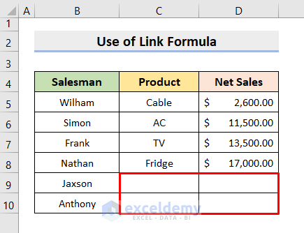
The source workbook is Book1 and the sheet name is X sheet.

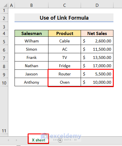
To fill the missing data in the red-colored box:

STEPS:

• Select C9 and enter the formula:

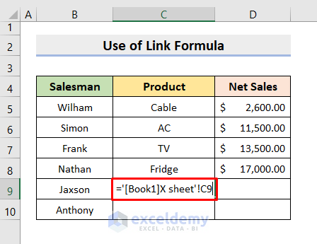
• Press Enter and use the AutoFill.
• Check Fill Without Formatting in the AutoFill Options to keep the format.

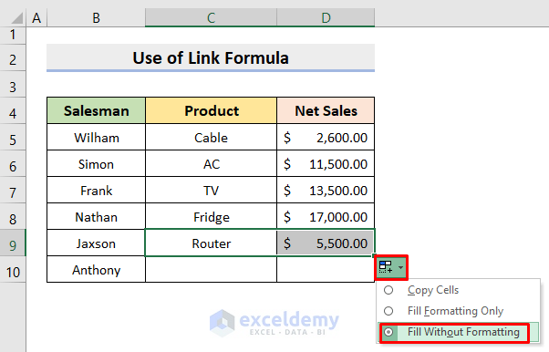
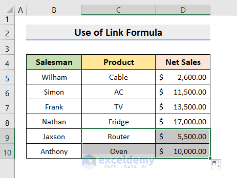
• Use the AutoFill to fill the rest of the missing data.

Method 2 – Using the Excel HYPERLINK Function to Link Sheets

There is missing data in D7. the HYPERLINK function will be used to see the cell value in the source worksheet: HYPERLINK1.

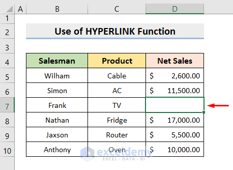
STEPS:

• Select D7 and enter the formula:

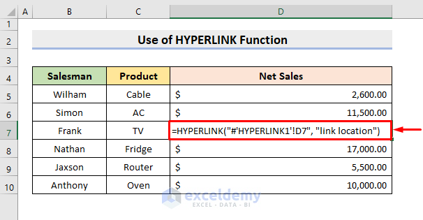
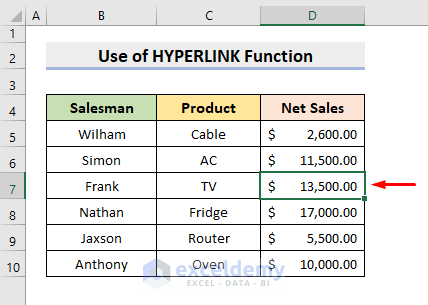
• Press Enter and you’ll see the link location underlined in blue.

• Press the link location to go to the source worksheet.

Read More: How to Link Cell to Another Sheet in Excel

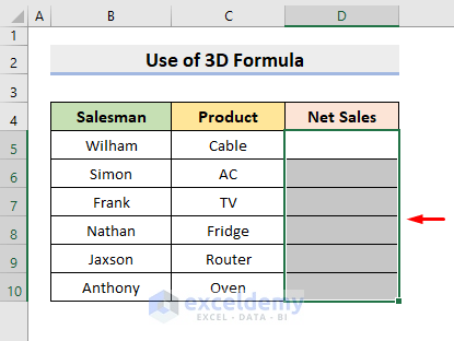
Method 3 – Linking Sheets with an Excel 3D Formula

To find the total of Net Sales by adding the values from sheets sheet1 and sheet2, use an Excel 3D Formula to link to other sheets and calculate the Sum.

STEPS:

• Select D5 and enter the formula:

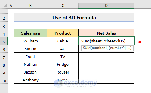
• Press Enter and use the Fill Handle to fill the series.

This is the output.

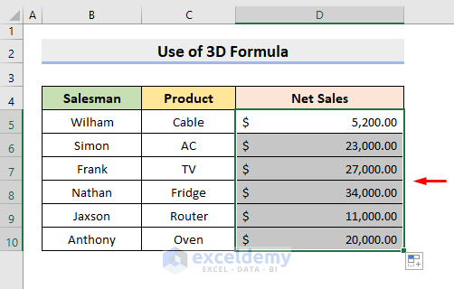
If you have a Space in your worksheet title, you have to change the formula:

STEPS:

• Select D5.
• Enter the formula:

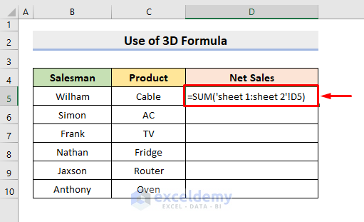
• Press Enter and use the AutoFill.

Read More: How to Link Data in Excel from One Sheet to Another

Method 4 – Using the SUM Formula to Link Sheets in Excel

The SUM summary sheet will be linked with sheet3 and sheet4 and D5 values in sheets sheet3 and sheet4 will be added, usingthe SUM Formula.

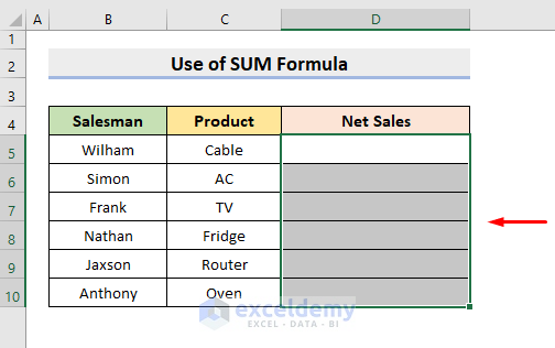
STEPS:

• Select D5.
• Enter the formula:

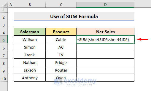
• Press Enter and use the Fill Handle to fill the rest of the cells.
• This is the output.

Download Practice Workbook

Download the following workbook to practice.

Related Articles

• How to Link Excel Data Across Multiple Sheets
• How to Link Sheets to a Master Sheet in Excel
• How to Link a Table in Excel to Another Sheet

<< Go Back To Excel Link Sheets | Linking in Excel | Learn Excel