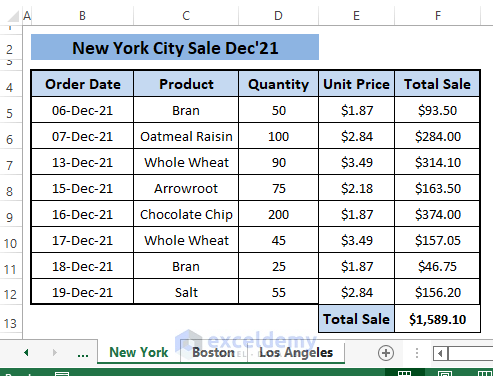
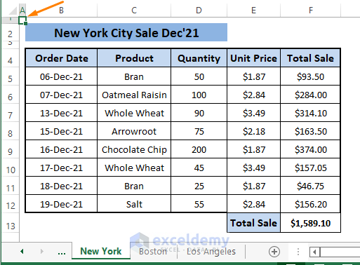
Let’s say we have sales data for three different cities, New York, Boston, and Los Angeles. These three are identical in form, so we’ll show only one worksheet as a dataset. We want to link these city sale sheets to a master sheet.
How to Link Sheets in Excel to a Master Sheet: 5 Easy Ways
Method 1 – Using the HYPERLINK Function to Link Sheets to a Master Sheet in Excel
The syntax of the HYPERLINK function is:
HYPERLINK (link_location, [friendly_name])link_location is the path to the sheet you want to jump.
[friendly_name] displays text in the cell where we insert the hyperlink [Optional].
Steps:
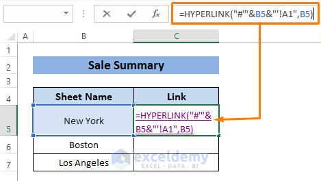
- Copy the following formula in any cell (i.e., C5).
=HYPERLINK("#'"&B5&"'!A1",B5)If we compare the arguments,
“#'”&B5&”‘!A1″= link_location
B5=[friendly_name]
- Press Enter and drag the Fill Handle to make the other hyperlinks appear in cells C6 and C7.
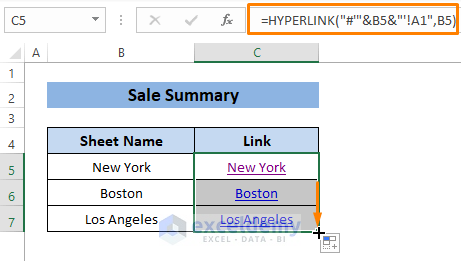
- You can see the hyperlinks for Boston and Los Angeles appear as they did for New York.
- You can check whether the hyperlinks work by clicking on them. We clicked on the New York named hyperlink.
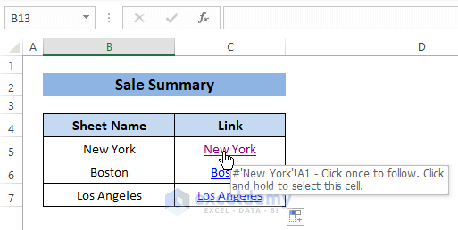
- Excel jumps to the New York sheet’s A1 cell (as directed in the formula) as shown in the image below.
Read More: How to Link Cell to Another Sheet in Excel
Method 2 – Using a Reference in a Formula to Link Sheets to a Master Sheet in Excel
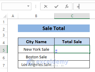
Let’s link only the Total Sale value from each city sheet in the master sheet.
Steps:
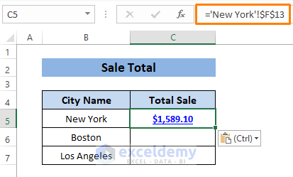
- Type the Equals Sign (=) in the formula bar.
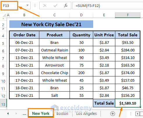
- Go to the respective sheet (i.e., New York) you want to reference a cell from.
- Select the Total Sale cell (i.e., F13) as a reference.
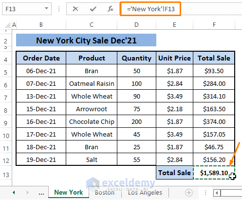
- Hit Enter.
- Repeat the process for the other two cells.
You can use the Context Menu to do the same job.
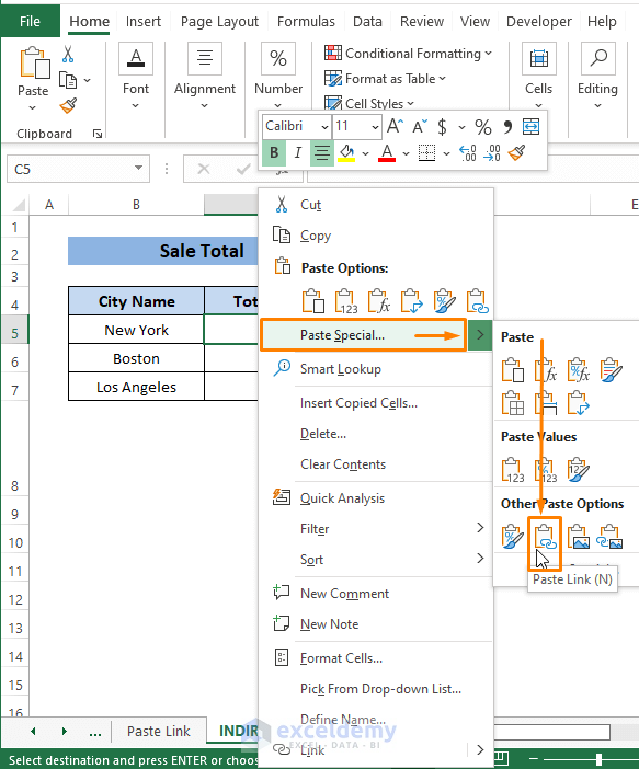
- Right-click on the cell you want to reference, then select Copy.

- Go to the Master sheet and right-click on the cell where you want to insert the value.
- Choose Paste Special, then select Paste Link (from Other Paste Options).
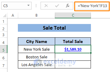
- You’ll see the sum value as shown in the following picture.
- You can repeat this for the other cells.
Read More: How to Reference Cell in Another Excel Sheet Based on Cell Value
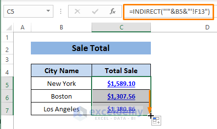
Method 3 – Using the INDIRECT Function to Link Sheets into a Master Sheet in Excel
The syntax of the INDIRECT function is:
INDIRECT (ref_text, [a1])The arguments refer,
ref_text; reference in the form of text.
[a1]; a boolean indication for A1 or R1C1 style reference [Optional]. Default represents TRUE=A1 style.
Steps:
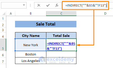
- Input the following formula in the first cell (i.e., C5):
=INDIRECT("'"&B5&"'!F13")We know the cell reference for the sum of Total Sale is in F13 for all three sheets and that B5 contains the sheet name from where the data will be fetched.
- Press Enter and drag the Fill Handle to the other cells.
Read More: How to Link Sheets in Excel with a Formula
Method 4 – Using a Name Box to Link Sheets to a Master in Excel
Steps:
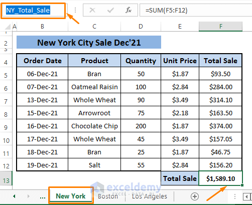
- Assign a name (i.e., NY_Total_Sale) for cell F13 in each city sheet using the Name Box.
- Repeat the step for other sheets such as Boston and Los Angeles.
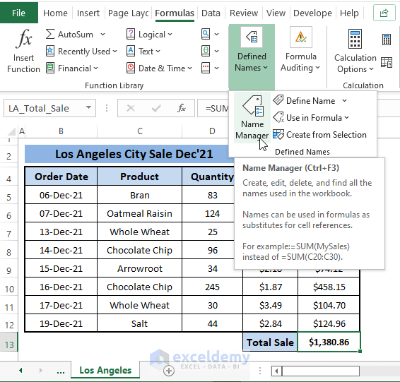
- To check the names, go to the Formulas tab and select Name Manager (from the Defined Names section).
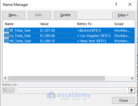
- The Name Manager window pops up and you can find all the assigned names in the workbook.
- Go to the master sheet.
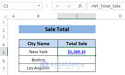
- Type =NY… to insert the sum value from the New York sheet. You’ll see the assigned name as a selectable option. Select the option.

- When you select the option, the sum of the Total Sale (for New York) value appears in the cell.
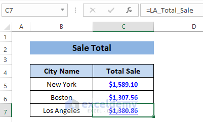
- Repeat this for other cities, and you’ll get all the values for respective cities as shown in the following image.
Read More: How to Link Two Sheets in Excel
Method 5 – Using the Paste Link Option to Link Sheets to a Master Sheet in Excel
Steps:
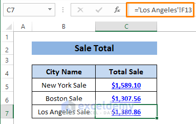
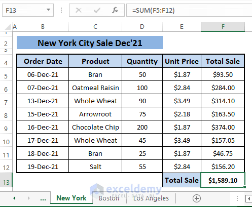
- First, identify the cell that you want to insert the link. The cell is F13 of the New York sheet. You have to repeat the steps for each sheet.
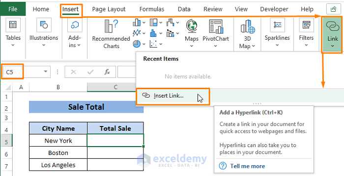
- In the master sheet, select the cell (i.e., C5) where you want to insert the link.
- Go to the Insert tab and select Insert Link (from the Link section).
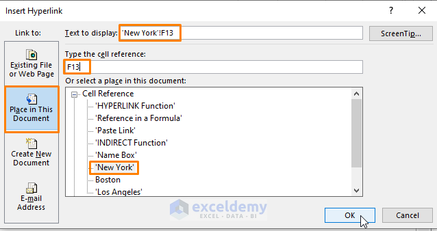
- The Insert Hyperlink window opens up. Select Place in the Document (under Link to options).
- Type F13 (in the Type the cell reference option)
- Select ‘New York’ (under Or select a place in this document)
- You’ll see ‘New York’!F13 as Text to display.
- Click OK.
- This inserts the link in the cell similar to the image below. If you want to check the link, click on it.
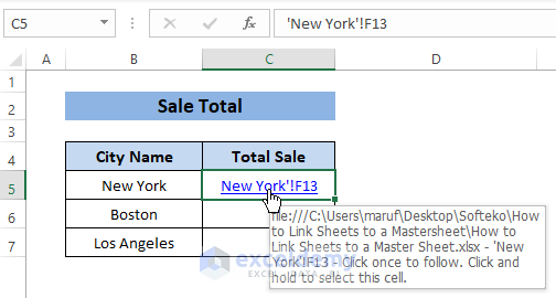
- The first link takes you to the New York sheet where the value sits.
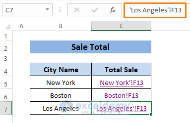
- Repeat the steps for the other cells.
Read More: How to Link Data in Excel from One Sheet to Another
Download the Workbook
Related Articles
<< Go Back To Excel Link Sheets | Linking in Excel | Learn Excel
Get FREE Advanced Excel Exercises with Solutions!
