How to Link Two Sheets in Excel – 3 Methods

Method 1 –  Using a Formula to Link Two Worksheets in Excel

There are two Excel sheets:  Destination Sheet and Source Sheet.

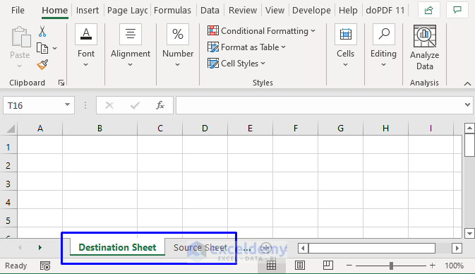
There is data in the Source Sheet that will be move to the Destination Sheet by linking the two sheets.

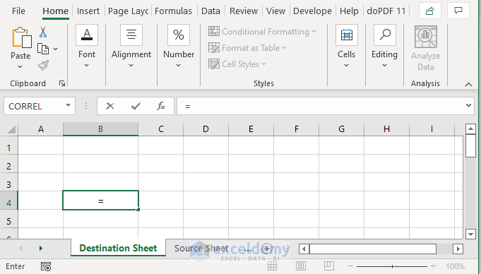
• In the Destination Sheet, select a cell (here, B4) and enter an equal sign (=).

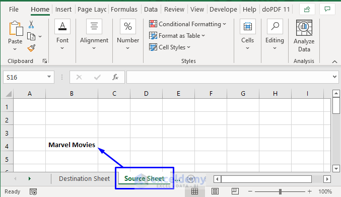
• Click the Source Sheet and the data (Marvel Movies in B4) that you want to retrieve in the Destination Sheet. You will see the whole formula in the formula bar.

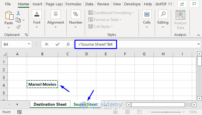
• Press Enter.

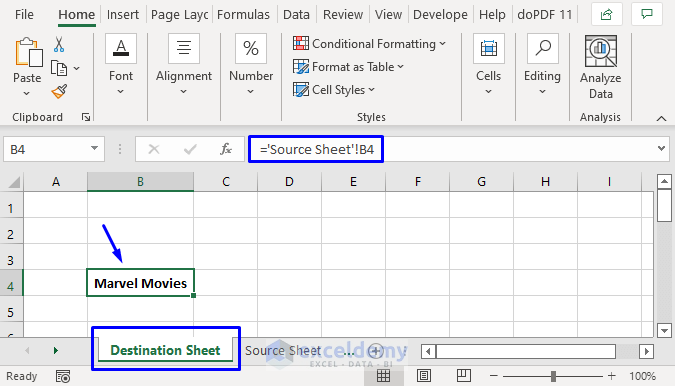
You will have the Source Sheet linked to the Destination Sheet .

Read More: How to Link Sheets in Excel with a Formula

Method 2 – Using the Copy-Paste Option to Link Two Excel Sheets

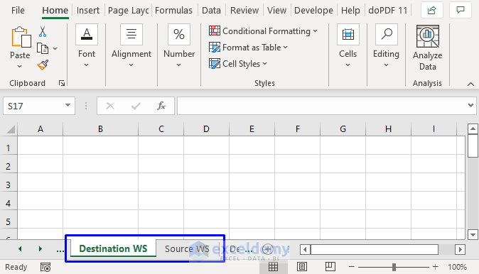
In the Source WS, there is DC Movies in B4.

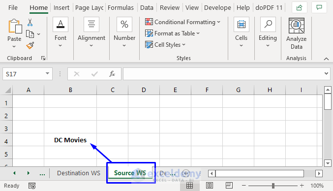
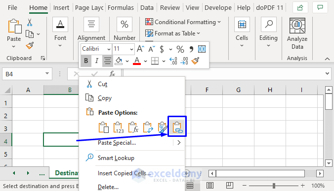
• Copy the data in Source WS.

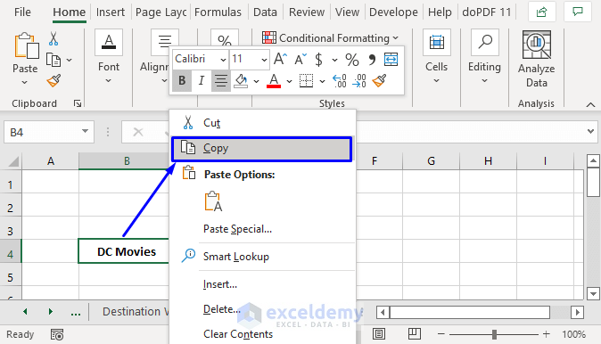
• Go back to Destination WS and click the cell in which you want to place the copied data.
• In that cell (B4, here), right-click and select Paste Link.

Data will be copied from Source WS into the Destination WS through a link.

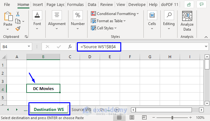
If you click the copied cell in Destination WS, you will see the formula in the formula bar.

Read More:  How to Link Excel Data Across Multiple Sheets

Method 3 –  Linking Two Excel Worksheets Manually

Create a formula to link one sheet to another:

equal sign (=) -> sheet name -> exclamatory mark (!) -> cell reference

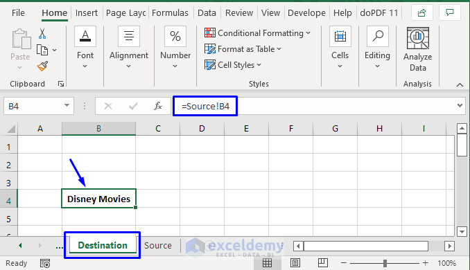
The image showcases two worksheets: Destination and Source.

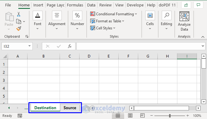
Source contains data that will be copied through a link into Destination by entering a formula manually.

• In Destination, select a cell (here, it B4).
• Enter the formula:

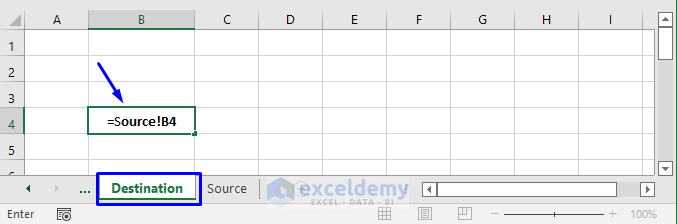
• Press Enter.

Data from Source is copied into Destination.

In linking formulas, if you add spaces and special characters, they must be wrapped in single quotes:

Read More: How to Link Data in Excel from One Sheet to Another

Download Workbook

Download the free practice Excel workbook here.

Related Articles

• How to Link Cell to Another Sheet in Excel
• How to Link Sheets to a Master Sheet in Excel
• How to Link a Table in Excel to Another Sheet

<< Go Back To Excel Link Sheets | Linking in Excel | Learn Excel