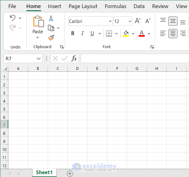
Step 1 – Creating a Dataset in Different Sheets
- Open a new Excel File.
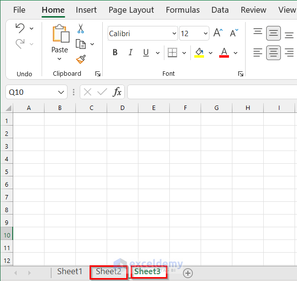
- Add two sheets: Sheet1 and Sheet2.
- Enter data in Sheet1.
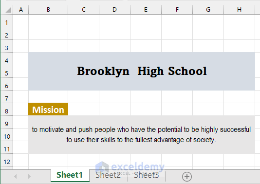
- Press ENTER.
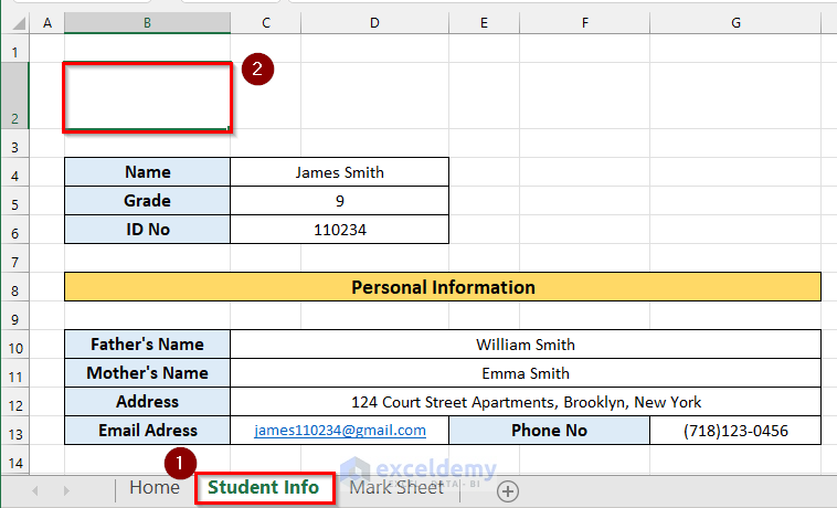
- Go to Sheet2 and enter data.
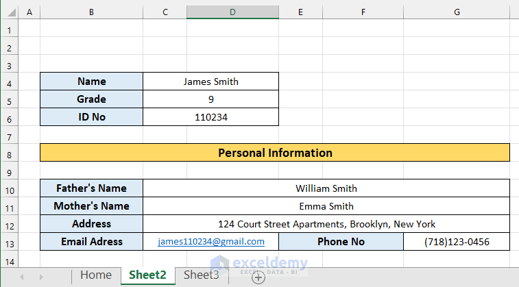
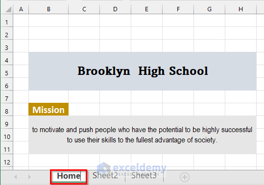
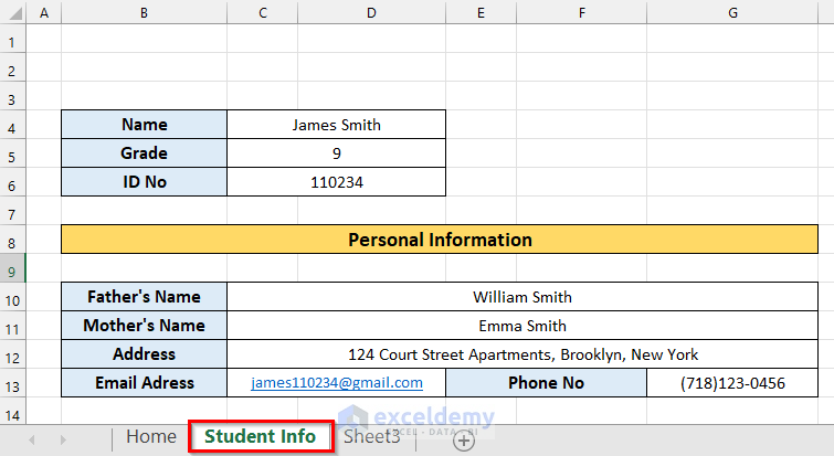
- Change the sheet name to Student Info following the steps described above.
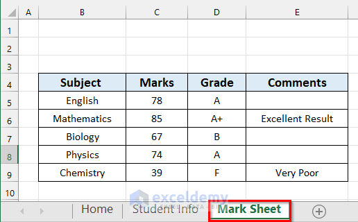
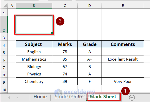
- Go to Sheet3 and enter data.
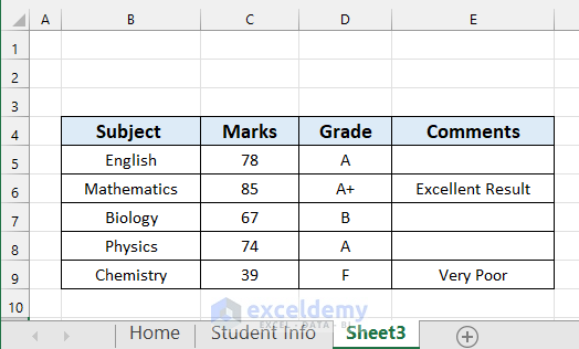
- Change the sheet name to Mark Sheet following the steps described above.
Step 2 – Inserting and Naming a Rectangular Box
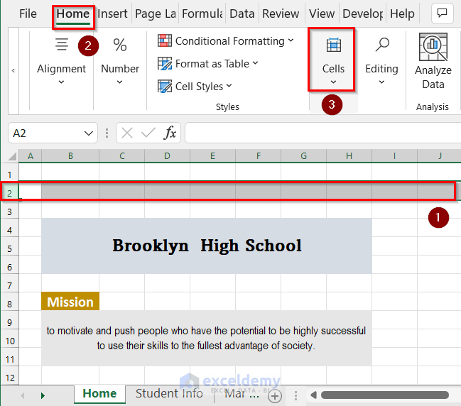
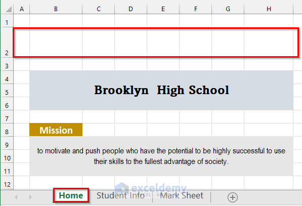
- Select row 2.
- Go to the Home tab >> click Cells.
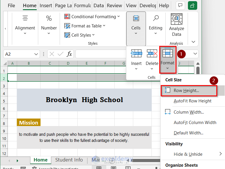
- Click Format >> select Row Height.
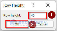
- Set 45 as Row height.
- Click OK.
- The row height of Row 2 changed.
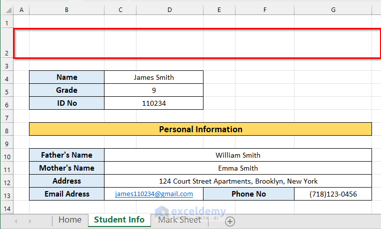
- Change the row height of Row 2 in Student Info.
- Change the row height of Row 2 in Mark Sheet.

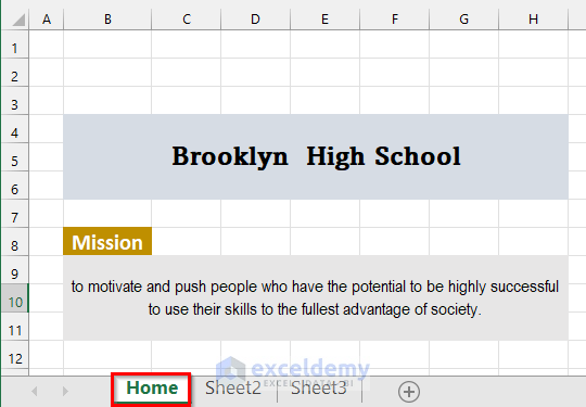
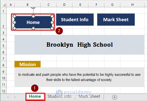
- Go to the Home sheet .
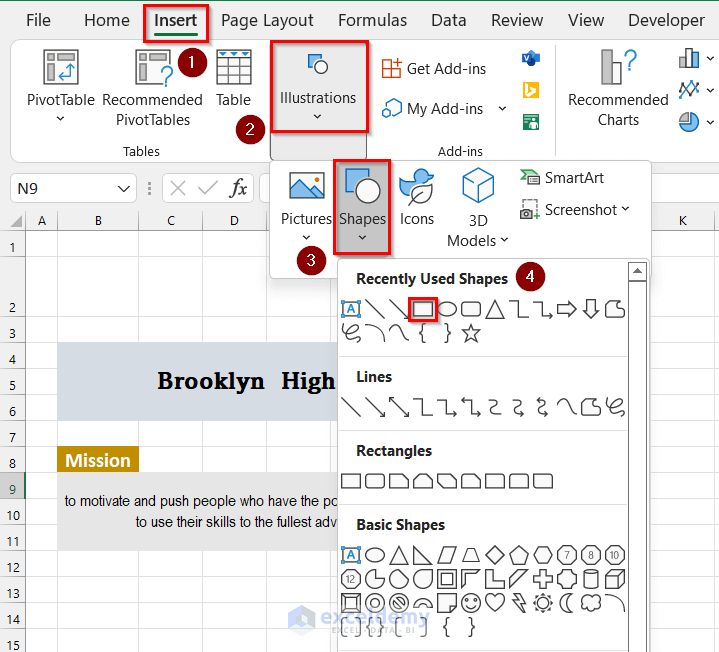
- In the Insert tab >> click Illustrations >> click Shapes >> select Rectangle.
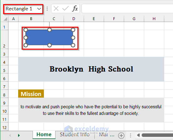
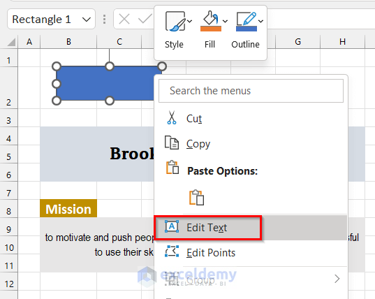
- Add a Rectangle to the Home sheet and right-click it.
- Select Edit Text.
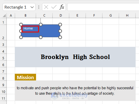
- Enter Home as text in the Rectangle.
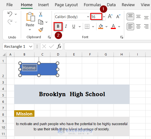
- Set 16 as Font Size.
- Click Bold.
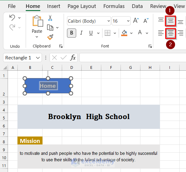
- Set Middle Align and Center as Alignment.
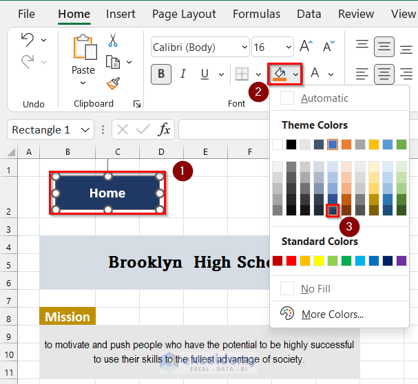
- Select the shape again.
- In Fill Color >> select Blue, Accent 1, Darker 50%.
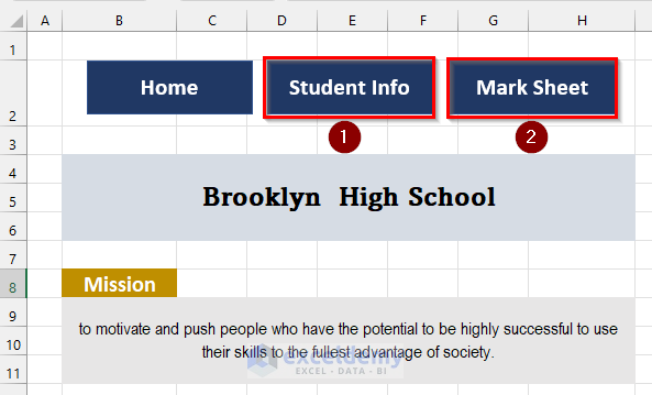
- Add 2 other rectangles and name them as Student Info and Mark Sheet following the steps described above.
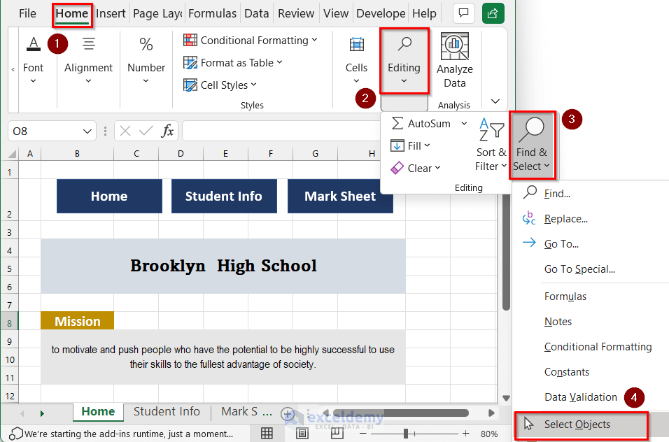
- In the Home tab >> click Editing >> click Find & Select >> select Select Objects.
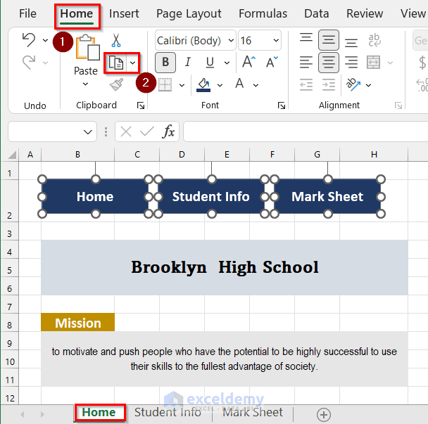
- Select the 3 Rectangles.
- Go to the Home tab >> click Copy.
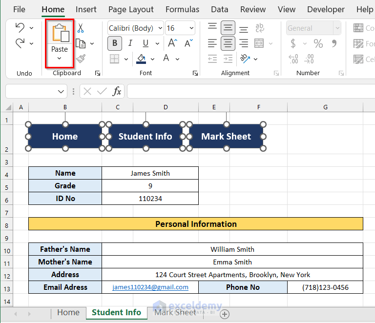
- Go to Student Info.
- Select B2.
- Click Paste.
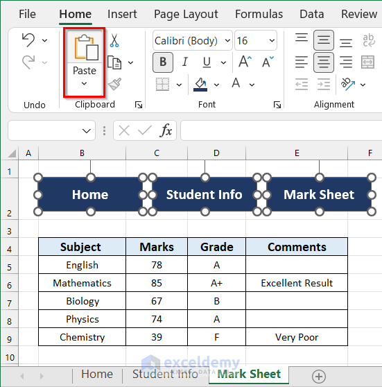
- Go to Mark Sheet.
- Select B2.
- Click Paste.
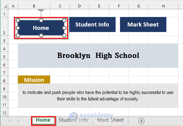
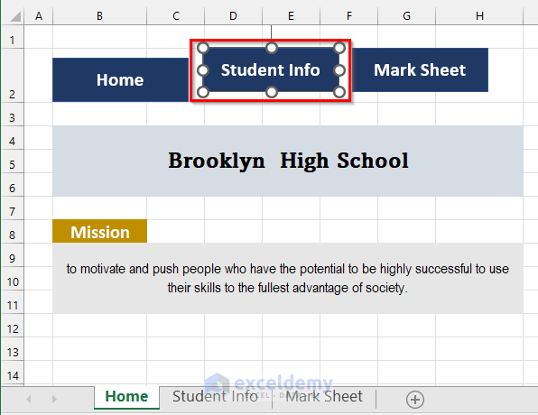
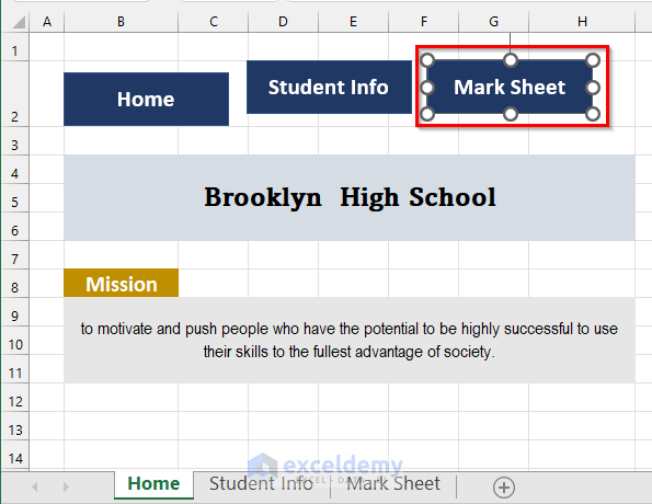
- Go to the Home sheet.
- Select the Home rectangle and drag it slightly down.
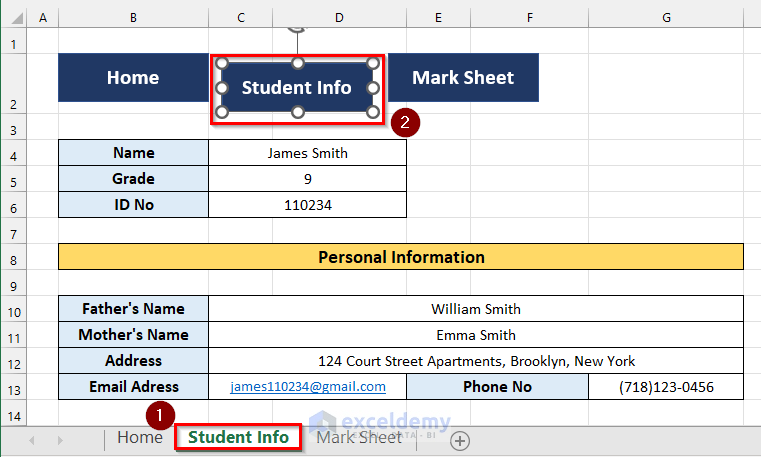
- Go to Student Info.
- Select the Student Info rectangle and drag it slightly down.
- Go to Mark Sheet.
- Select the Mark Sheet rectangle and drag it slightly down.

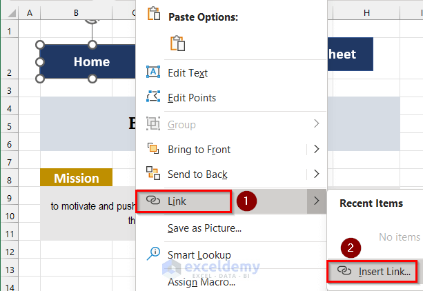
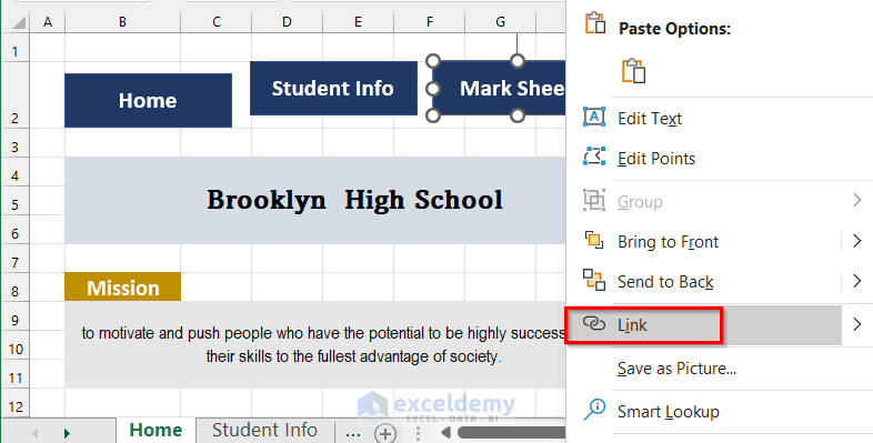
Step 3 – Creating a Link Between Sheets to Make Excel Look Like an Application
- Click Link >> select Insert Link.
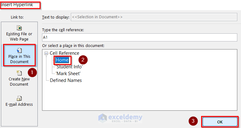
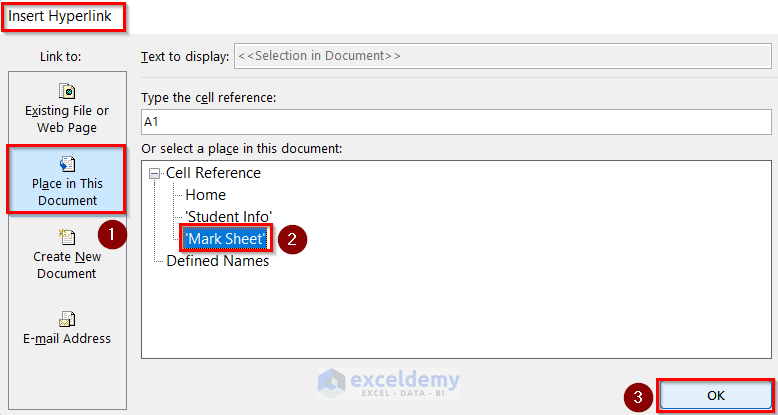
- In the Insert Hyperlink box, click Place in this Document >> select Home.
- Click OK.
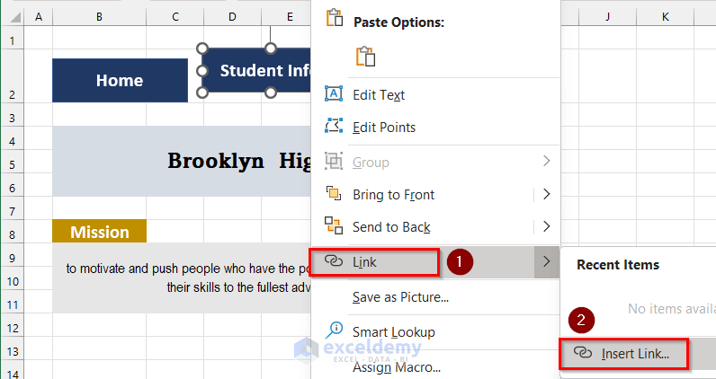
- Select the Student Info rectangle.
- Right-click it.
- Click Link >> select Insert Link.
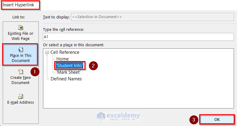
- In the Insert Hyperlink box, click Place in this Document>> select Student Info.
- Click OK.
- Select the Mark Sheet rectangle.
- Right-click it.
- Click Link >> select Insert Link.
- In the Insert Hyperlink box, click Place in this Document >> select Mark Sheet.
- Click OK.
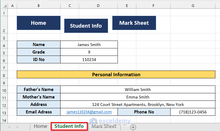
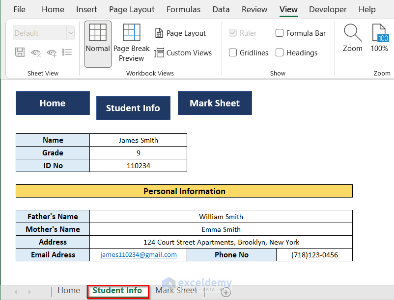
- Go to Student Info.
- Create links between the sheets following the steps described above.
- Go to Mark Sheet.
- Create links between the sheets following the steps described above.
Step 4 – Hiding Headings, Formula Bar, Ribbon and Sheet Tabs to Make Excel Look Like an Application
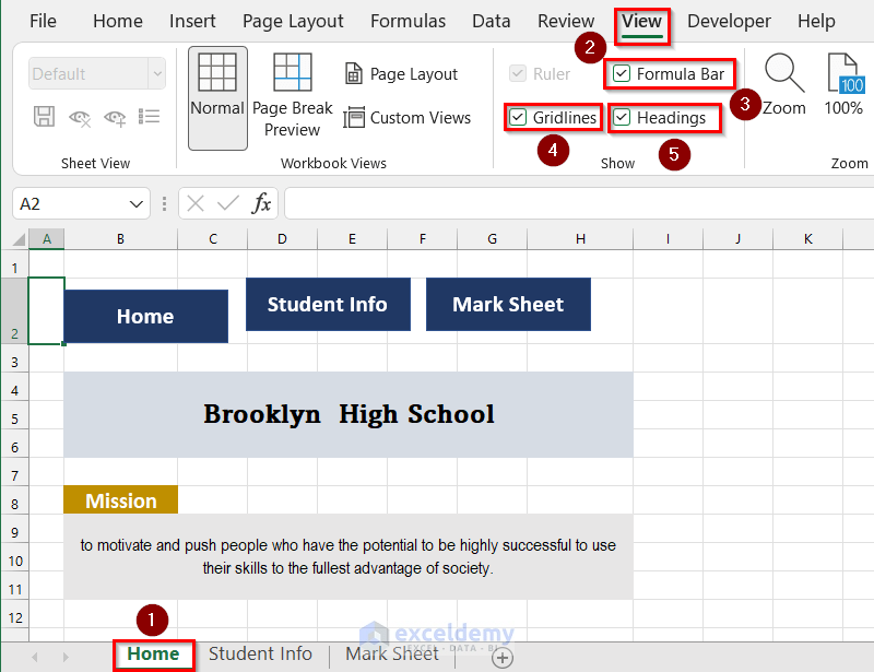
- Go to the Home sheet.
- In the View tab >> uncheck Formula Bar, Gridlines, and Headings.
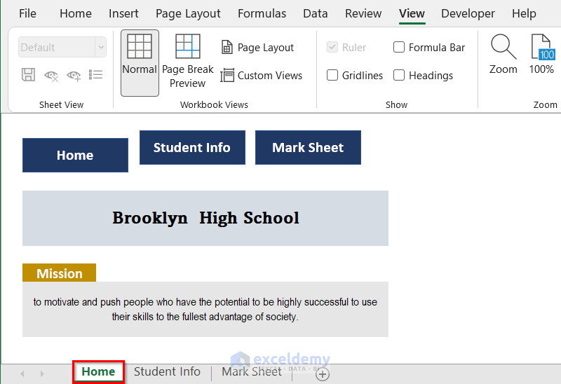
- This is the output.
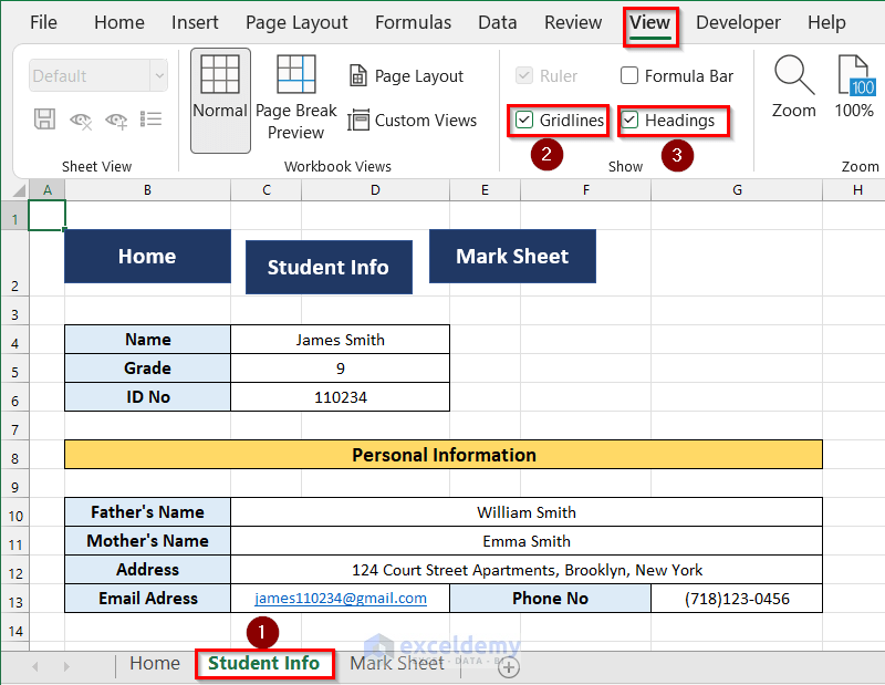
- Go to Student Info.
- Go to the View tab >> uncheck Gridlines, Headings.
- This is the output.
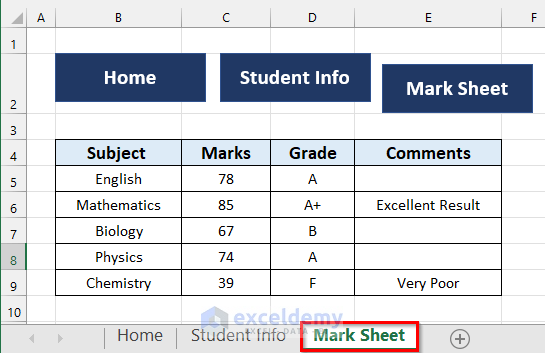
- Go to Mark Sheet.
- In the View tab >> uncheck Gridlines, Headings.
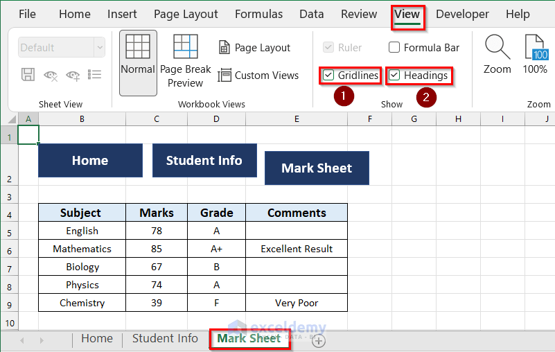
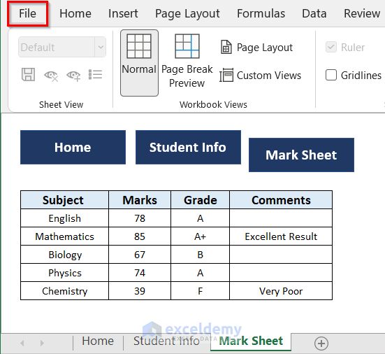
- This is the output.

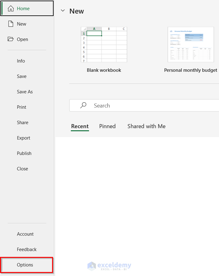
- Click the File tab.
- Select Options.
- In the Excel Options box, go to Advanced.
- Uncheck Show sheet tabs.
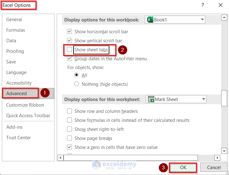
- This is the final output.

Download Practice Workbook
Related Articles
- How to Automatically Update One Worksheet from Another Sheet in Excel
- Transfer Data from One Excel Worksheet to Another Automatically
- How to Reference Cell in Another Excel Sheet Based on Cell Value
- Transfer Specific Data from One Worksheet to Another for Reports
- Linking Excel Sheets to a Summary Page
<< Go Back To Excel Link Sheets | Linking in Excel | Learn Excel
Get FREE Advanced Excel Exercises with Solutions!

A good tip to finish this off is to select the column after the last populated column of your sheet, then Ctrl+Shift+Right to select all columns, then right click and hide those columns. Do the same with the rows below your data.
The only thing I’d like to work out now is how to get it sort of centre aligned in the screen, and hide the Formula bar and Ribbon (I know this can be done, but only on the local machine, and then it’s missing for every other spreadsheet you use in Excel too).
Hi EDD,
Thanks for your comment. Hiding the Formula bar and Ribbon are typically done on a per-workbook basis and aren’t usually carried over to other workbooks you open. However, when you hide Formula Bar and Ribbon from any specific worksheet of your workbook, they’ll be removed from all the other worksheets of that workbook.
You can follow a manual process to align the range in the center of the screen. To center align all the elements on the screen, select the whole range and press Ctrl + X to cut the total range. Here, for the Home page, we will cut cell range B1:H12.
Then, press Ctrl + V to paste it in the center of your screen.
Similarly, you have to cut and paste all the elements to the center and align them on the screen manually.
We hope this will solve your problem. Please let us know if you face any further problems.
Regards,
Arin Islam,
ExcelDemy