Example 1 – Select a Single Cell and Refer to a Whole Range of Cells
We have two sample Excel worksheets with the names AAPL and MSFT. Both worksheets have similar kinds of data. Profit (PCO), EPS, and Growth of two companies for the last 5 years.
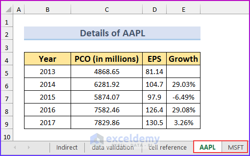
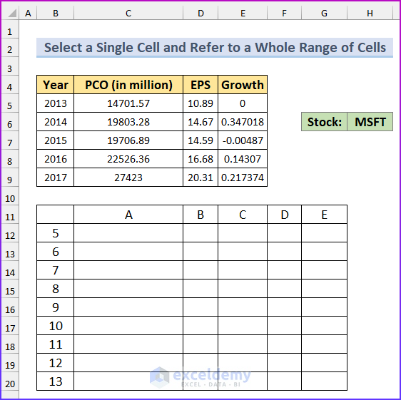
Our goal is to input the company name from a drop-down in the main worksheet and have all the other values ((Year, PCO, EPS, and Growth)) be displayed accordingly.
This method can be helpful if you’re maintaining the same kind of data across hundreds of worksheets. We will use a formula like this:
=INDIRECT('worksheet_name'!column_reference&row_reference)
Steps:
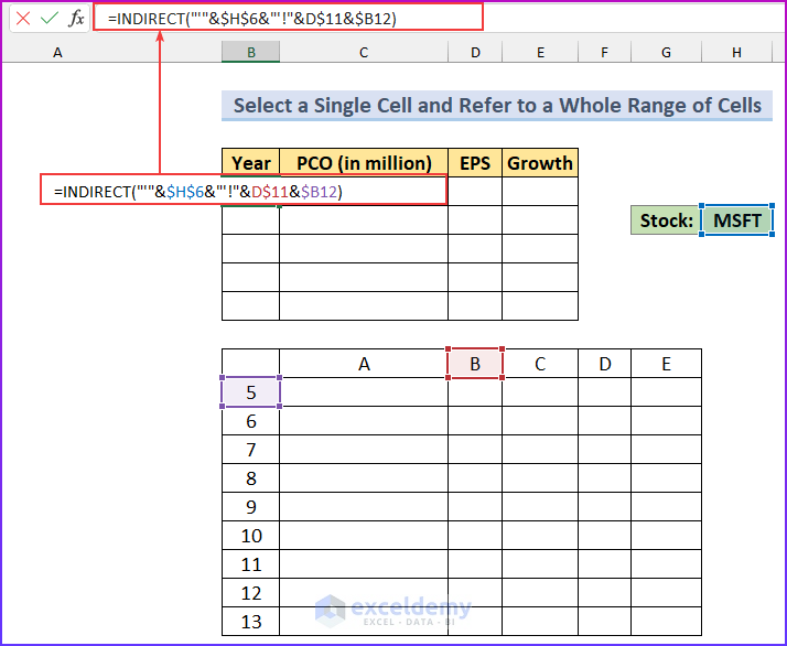
- For column_reference, cell range: C11:G11. This range holds values from A to E. You can extend it as required. For row_reference, cell range: B12:B16. This range holds values from 5 to 13. Extend it as required.
- We used the formula below in cell B5 of the main worksheet:
=INDIRECT("'"&$H$6&"'!"&D$11&$B12)
- Apply this formula to other cells in the range (B5:E9).
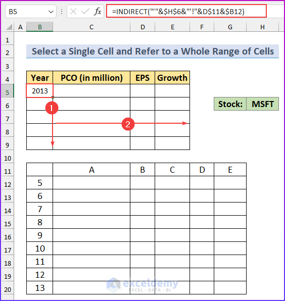
- This is the result you will get:
Formula Breakdown
- (“‘”&$H$6&”‘!”) returns the worksheet name “MSFT!'” (for the above image).
- &D$11 refers to cell reference D11 and returns the text value &”B”.
- &$B12 refers to cell reference B12 and returns the numeric value &5.
- The overall return from the 3 parts of the formula: “‘MSFT!'”&”B”&5 = “‘MSFT!’B5”
Notes: When a text value and a numeric value are concatenated in Excel, the return is a text value.
- The ultimate return of the formula: INDIRECT(“MSFT!’B5”)
- When we apply the formula to other cells in the range, it works because we have used mixed cell references like D$11 and $B12. When the formula is applied to the cells on the right, only the column references change, for reference D$11. When the formula is applied to the cells on the bottom, only row references change for reference $B12.
Notes: To see how the different parts of an Excel formula work, select any part and press the F9 key. You will see the value of that part of the formula.
Read More: How to Link Cell to Another Sheet in Excel
Example 2 – Reference Individual Cell of Another Worksheet
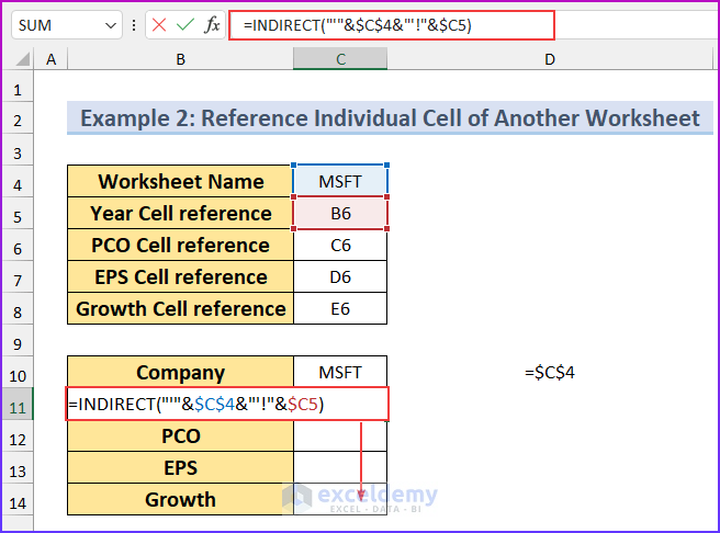
In this example, we will pull a row from another worksheet based on some cell values (references).
Steps:
- We created our sample dataset.
- Use the formula below in cell C10.
=$C$4
- Add this formula in cell C11.
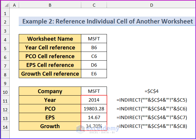
=INDIRECT("'"&$C$4&"'!"&$C5)
- AutoFill the formula for the cell range C11:C14.
- The worksheet will look like this.
Read More: How to Link Data in Excel from One Sheet to Another
Download Excel Workbook
Related Articles
- How to Automatically Update One Worksheet from Another Sheet in Excel
- Transfer Data from One Excel Worksheet to Another Automatically
- Transfer Specific Data from One Worksheet to Another for Reports
- Linking Excel Sheets to a Summary Page
- How to Make Excel Look Like an Application
<< Go Back To Excel Link Sheets | Linking in Excel | Learn Excel
Get FREE Advanced Excel Exercises with Solutions!

Great Article!!! I can put this to use right now 🙂 It would be even more powerful if I knew how to pull a table of data in from another worksheet or, even better, another workbook without the cell reference table being used as reference… For example I have similarly formatted data that I want to chart using the drop down as you have already done. To have this reference table, even hidden, will distract the people I will present the data to…
Thanks for your feedback, JG. I will think about a method as per your necessity.
Best regards
Kawser
when a cell has a number (12345) that is ok but when the next cell has($123.45) how to get the decimal in
with out having to manual installing it.when there is ten cells part are numbers part are dollars.
i guess i will just put them ?
a b c d e
12 2 24 $1.99 $4.39
like this
jr
=SUM(sheetname1!cell reference, sheetname2!cell reference,…)