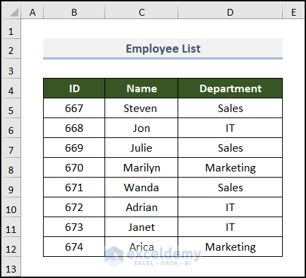
Let’s use an Employee List. This dataset includes the ID, Name, and Department in columns B, C, and D, respectively.
Method 1 – Using the Copy Command from the Ribbon
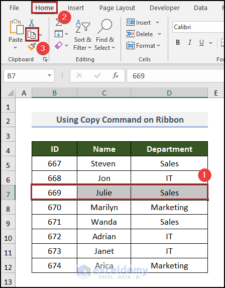
Let’s copy the cells in Row 7 which is the row with ID 669.
Steps:
- Select all cells in the B7:D7 range.
- Navigate to the Home tab.
- Click on the Copy icon in the Clipboard group of commands.
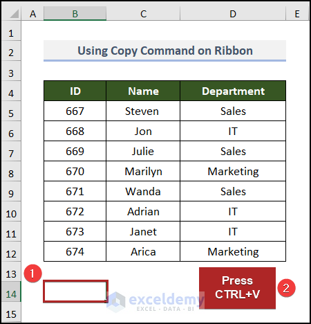
- Your selected row has been copied to the clipboard, and you are ready to paste it anywhere you want. Let’s paste it in cell B14.
- Go to cell B14 and press Ctrl + V to paste it.
- The row is copied to the desired location.

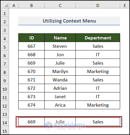
Method 2 – Utilizing the Context Menu
Steps:
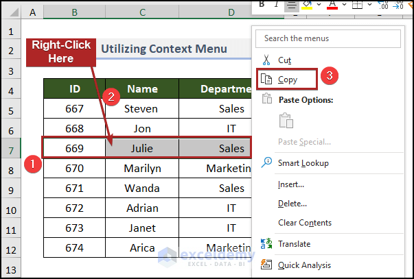
- Select cells B7:D7.
- Right-click while keeping the cursor anywhere inside the selection.
- Click on Copy.
- Select a destination cell and press Ctrl + V to paste the row.
Method 3 – Applying the Drag and Drop Method
Steps:
- Select the row.
- Move the pointer to the border of the selection area, so that the mouse pointer becomes a move pointer.
- Hold the Ctrl key and drag the selection area to a new location.
- Release Ctrl.
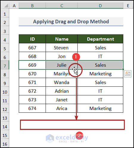
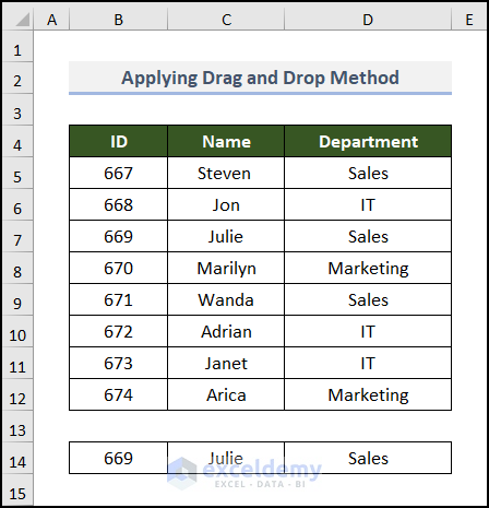
- Here’s how it looked when we copied row 7 to row 14.
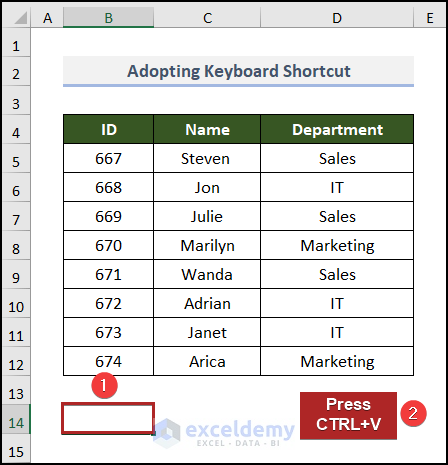
Method 4 – Keyboard Shortcuts
Steps:
- Select Row 7 (B7:D7).
- Press Ctrl + C.
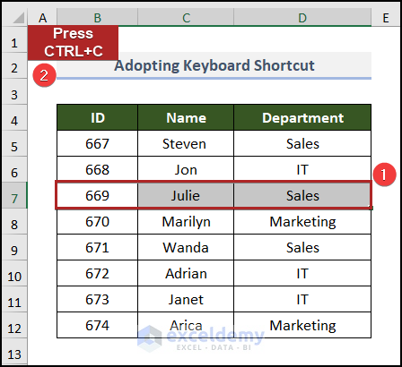
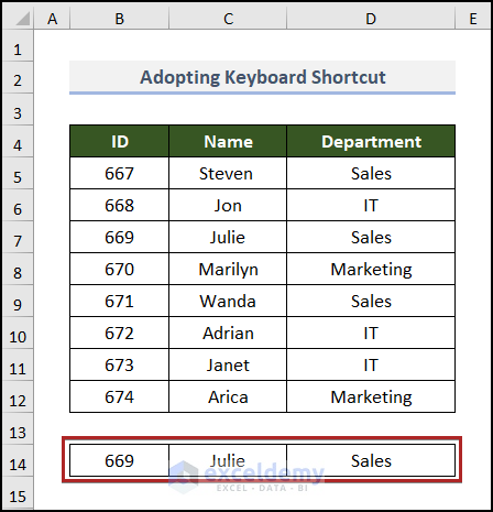
- Go to the destination cell and press Ctrl + V to paste the row.
- The row has been copied.
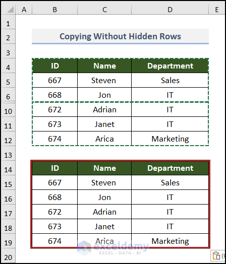
Method 5 – Copying Without Hidden Rows
There are some hidden rows in the dataset. Look at the image below.
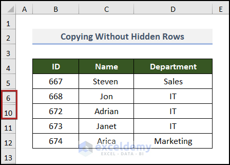
There are 3 rows hidden between Row 6 and Row 10. If you copy the range and paste it into cell B14 using Method 1, the output will be like the following.
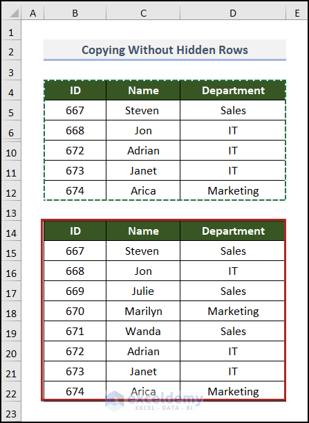
Let’s copy just the visible rows.
Steps:
- Select cells in the B4:D12 range.
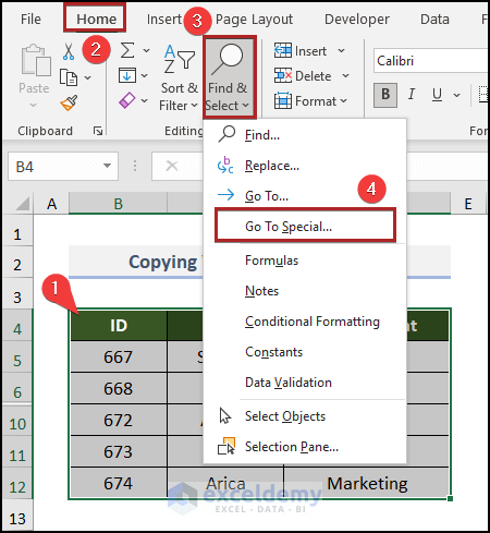
- Go to the Home tab.
- Click on the Find & Select drop-down icon on the Editing group.
- Select the Go to Special… option.
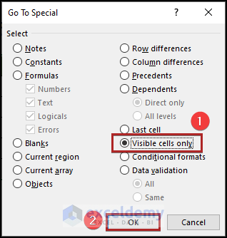
- The dialog box for the Go To Special command appears.
- Select Visible cells only.
- Click OK.
- Follow the previous methods to copy and paste the selection into a preferred location.
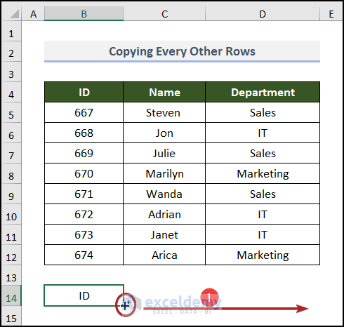
Method 6 – Copying Every Other Row
Steps:
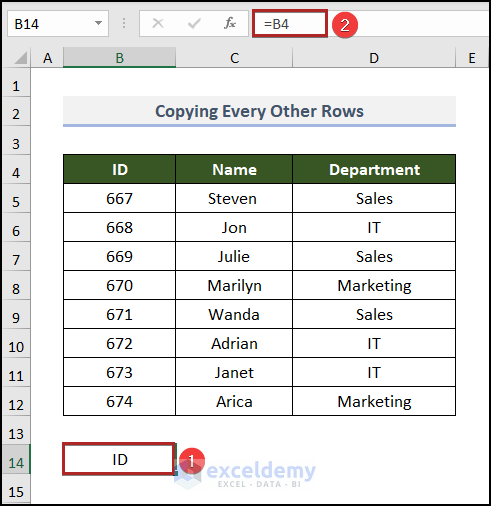
- Select cell B14 and enter the following formula:
=B4- Press Enter.
- Drag the Fill Handle horizontally to cell D14.
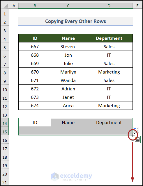
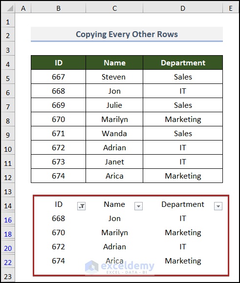
- Select cells in the B14:D15 range and drag the Fill Handle up to cell D22.
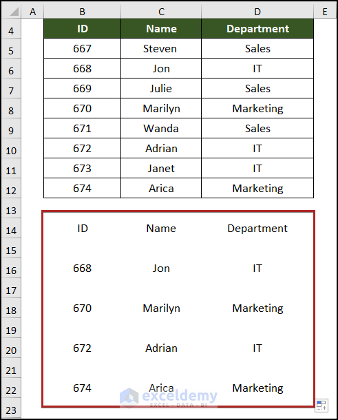
- The result will look like the following image.
- Select the new data range.
- Go to the Home tab.
- Click on the Sort & Filter drop-down.
- Choose Filter from the list.
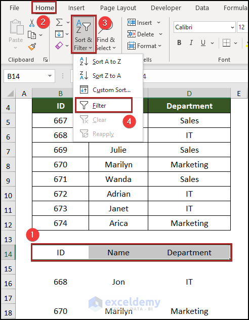
- Click on the Filter Button beside the heading ID.
- Uncheck the box Blanks and click OK.
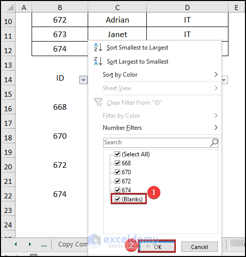
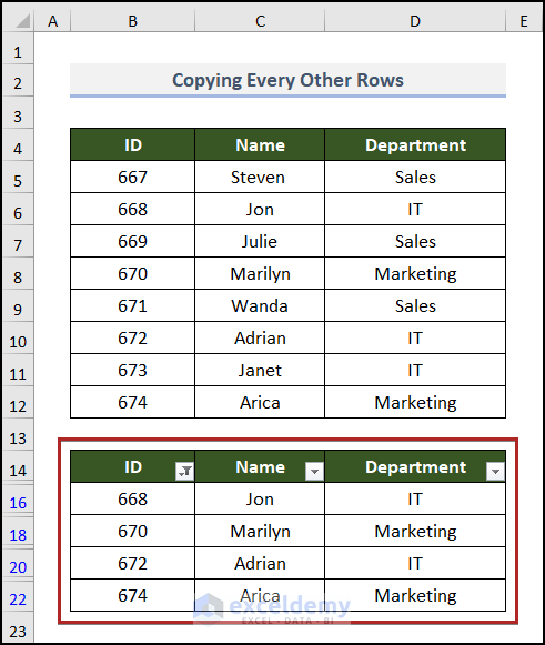
- The blank rows get removed.
- After a bit of formatting, the copied range looks like the following one.
Method 7 – Copying Rows with Formula
Steps:
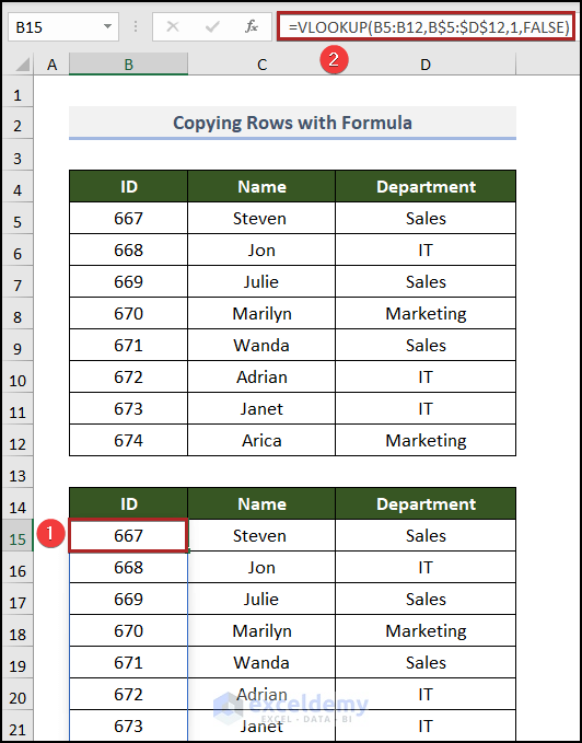
- Go to cell B15 and insert the formula below:
=VLOOKUP(B5:B12,B$5:$D$12,1,FALSE)Here, the VLOOKUP function returns the value of the same row from the specified column of the given table, where the value in the leftmost column matches the lookup_value.
- Press Enter.
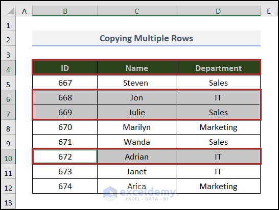
How to Copy Multiple Rows in Excel
Steps:
- Select any row.
- Hold the Ctrl key and select as many rows as you want.
- Release the Ctrl key when you are done selecting the rows.
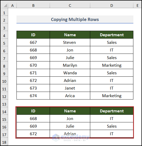
- Repeat the steps of Method 1 to copy and paste them.
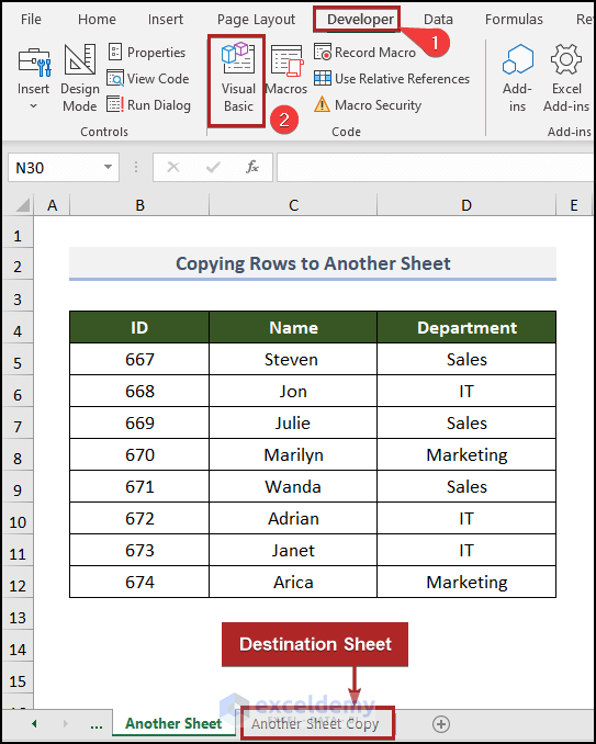
How to Copy Multiple Rows to Another Sheet in Excel
Steps:
- Go to the Developer tab.
- Click on the Visual Basic icon.
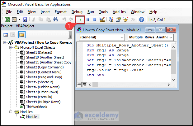
- The Microsoft Visual Basic for Applications window will open up.
- Jump to the Insert tab.
- Click on Module from the options.
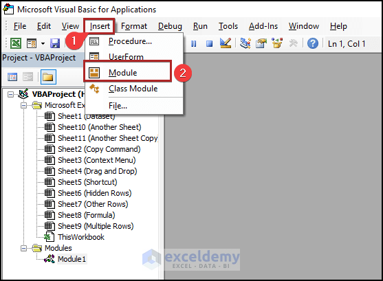
- Excel will insert a code module.
- Paste the following VBA code into the module:
Sub Multiple_Rows_Another_Sheet()
Dim rng1 As Range
Dim rng2 As Range
Set rng1 = ThisWorkbook.Sheets("Another Sheet").UsedRange
Set rng2 = ThisWorkbook.Sheets("Another Sheet Copy").Range(rng1.Address)
rng2.Value = rng1.Value
End Sub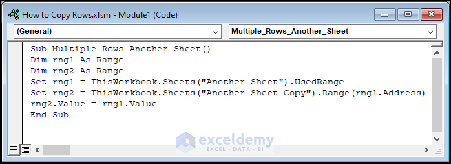
- Click on the Run button.
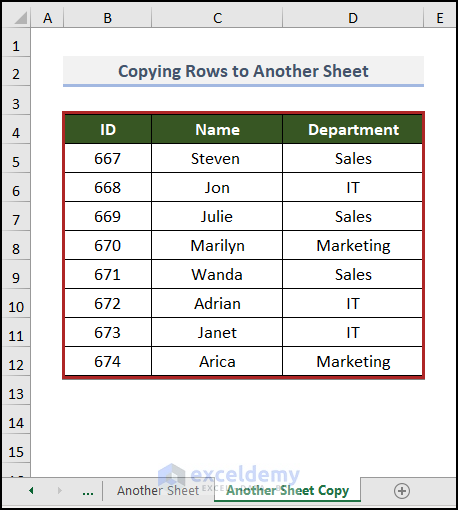
- The final result is on another sheet. You have to apply formatting manually.
Download the Practice Workbook
How to Copy Rows in Excel: Knowledge Hub
<< Go Back to Copy Paste in Excel | Learn Excel
Get FREE Advanced Excel Exercises with Solutions!
