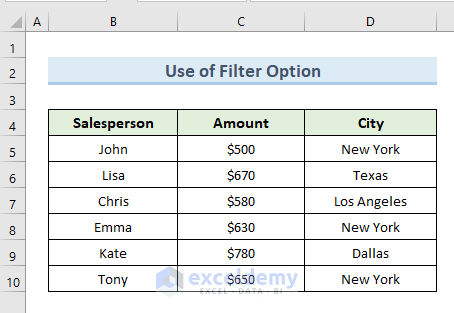
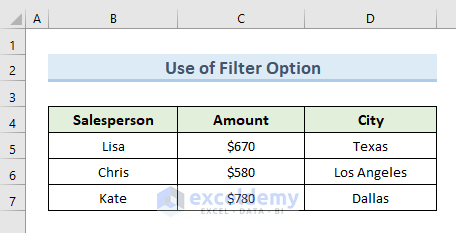
Method 1 – Automatically Copy Rows in Excel to Another Sheet Using Filters
In the following dataset, we will copy all rows from the data range (B4:D10) except the rows that contain New York in the City cell.
Steps:
- Select the entire data range (B4:D10).
- Go to the Data tab and choose Sort & Filter, then select Filter.
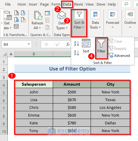
- The filter icons are now visible in the headers of the data range.

- Click on the drop-down icon in cell D4.
- Check only the option New York and uncheck the rest.
- Press OK.
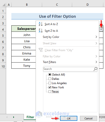
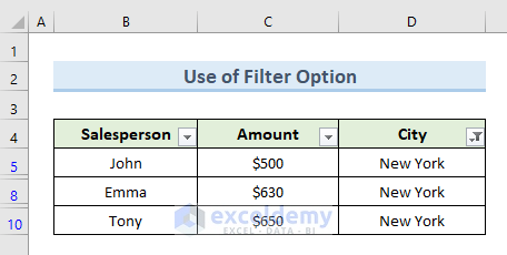
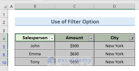
- We can see only the rows with New York.
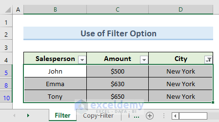
- Select the filtered data range (B4:D10) and press Alt +; to select all the visible cells.
- Right-click and select the option Copy or use the shortcut Ctrl + C to copy the selected data range.
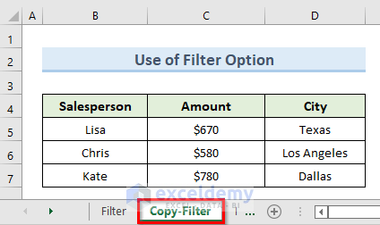
- Go to another sheet named “Copy-Filter” and paste the copied data.
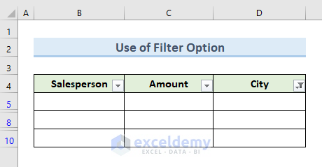
- Go back to the previous sheet, select cells (B5:D10), and delete them.
- There is no data visible in our worksheet now.
- Go to the Data tab and disable the filter option. We got the sales data of the city “New York” deleted from the data range.
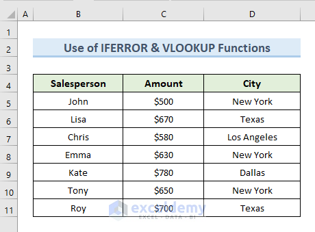
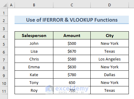
Method 2 – Combine IFERROR and VLOOKUP Functions to Copy Rows Automatically to Another Sheet in Excel
We will continue with the same dataset that we used in the previous example.
Steps:
- Go to the sheet “IFERROR &VLOOKUP(2)” (from our sample workbook) to paste the data.
- Select cell B4 and insert the following formula in that cell:
=IFERROR(VLOOKUP('IFERROR &VLOOKUP'!$B$4:$B$1000,'IFERROR &VLOOKUP'!$B$4:$D$1000,1, FALSE), "")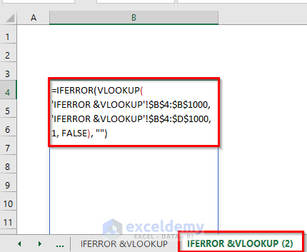
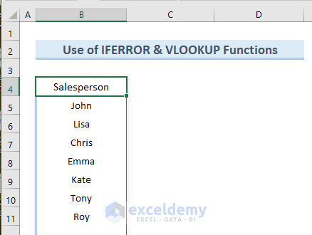
- Press Enter. The above command returns the values of column B from the sheet “IFERROR & VLOOKUP” in sheet “IFERROR &VLOOKUP (2)”.
- In cell C4, insert the formula:
=IFERROR(VLOOKUP('IFERROR &VLOOKUP'!$B$4:$B$1000,'IFERROR &VLOOKUP'!$B$4:$D$1000,2, FALSE), "")- In cell D4, insert the formula:
=IFERROR(VLOOKUP('IFERROR &VLOOKUP'!$B$4:$B$1000,'IFERROR &VLOOKUP'!$B$4:$D$1000,3, FALSE), "")- The above formulas will give you a dataset like the following image.
- Go back to the worksheet “IFERROR &VLOOKUP”.
- Add a new row in the data range like the highlighted one in the following image.
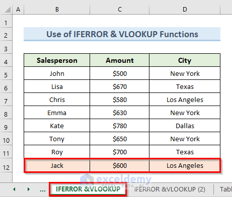
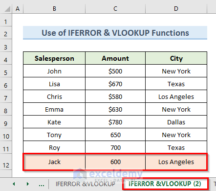
- Open the worksheet “IFERROR &VLOOKUP(2)”.
- The newly added row in the worksheet “IFERROR &VLOOKUP“ is duplicated into the worksheet “IFERROR &VLOOKUP(2)”.
How Does the Formula Work?
- VLOOKUP(‘IFERROR &VLOOKUP’!$B$4:$B$1000,’IFERROR &VLOOKUP’!$B$4:$D$1000,1, FALSE), “”): This part retrieve the values from the first column of the worksheet ‘IFERROR &VLOOKUP‘.
- IFERROR(VLOOKUP(‘IFERROR &VLOOKUP’!$B$4:$B$1000,’IFERROR &VLOOKUP’!$B$4:$D$1000,1, FALSE), “”): Returns blank if any VLOOKUP value in the range ($B$4:$D$1000) gives an error.
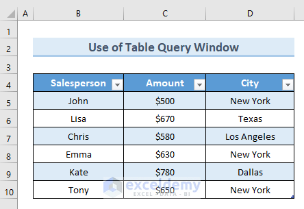
Method 3 – Insert a Table Query Window to Copy Rows Automatically in Excel to Another Sheet
We will continue with our previous dataset. However, we will use the table format of the data range like in the following image.
Steps:
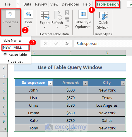
- Select the entire table range (B4:D10).
- Go to the Table Design tab and select the option Properties. Rename the table as “New_Table”.
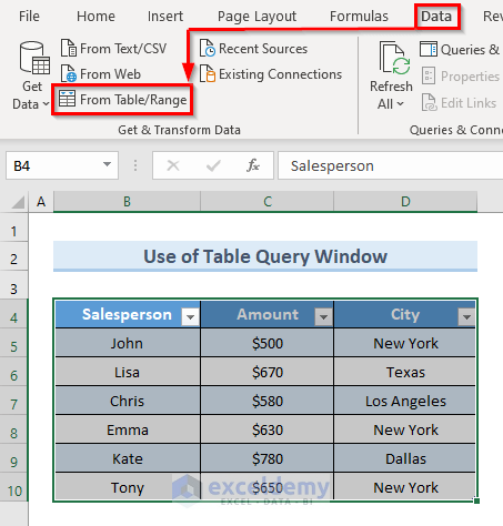
- Select the option From Table/Range from the ribbon of the Data tab.
- A new window will appear for query settings. Go to the Add Column tab in that window.
- From the drop-down of the Index Column, select the option From 1.
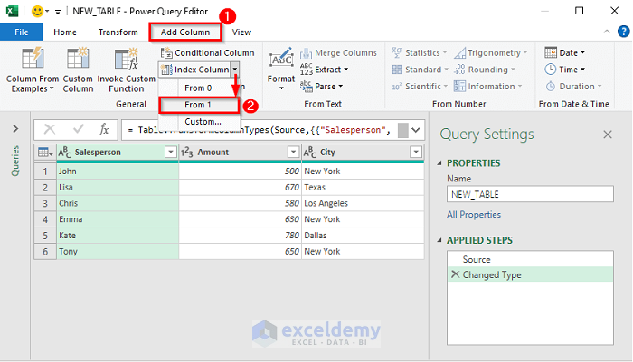
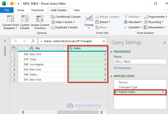
- This adds a new Index column in the existing data range.
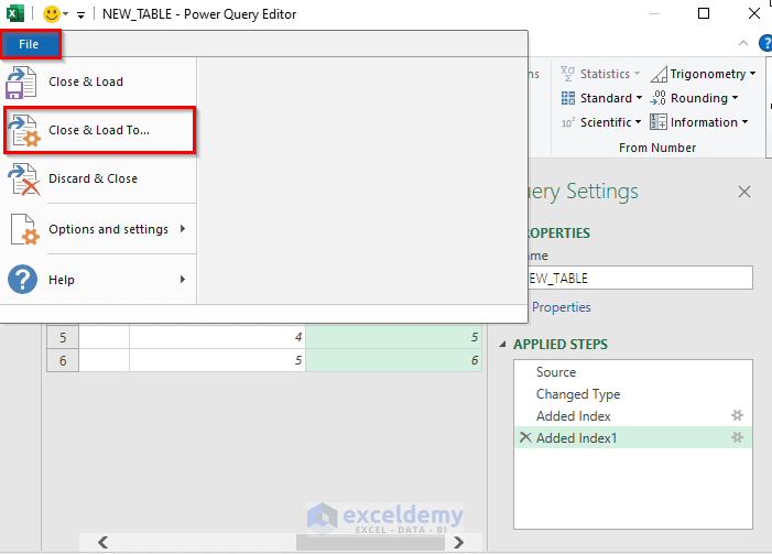
- Go to File.
- Click on the option “Close & Load To”.
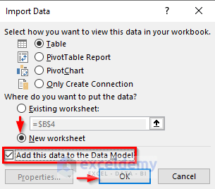
- One more dialogue box will appear. Check the option “New worksheet” to put the data in a new worksheet.
- Check the option “Add this data to the Data Model”.
- Press OK.
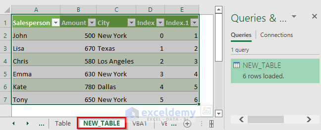
- This returns a new table in a new worksheet. The new worksheet’s name is the same as the table’s name.
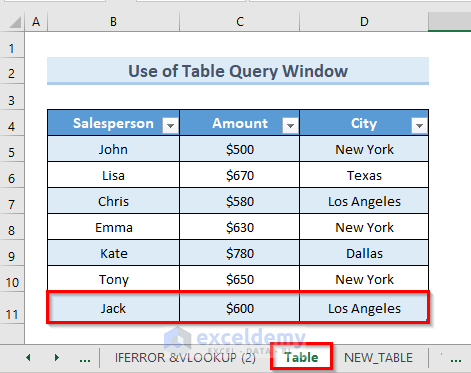
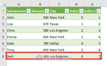
- Go back to the worksheet “Table”.
- Add a new row in the data range like the highlighted one in the following image.
- Go to the worksheet “NEW_TABLE”.
- Right-click on the name of the worksheet in the “Queries & Settings” section and click on “Refresh”.
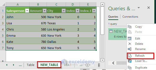
- If we add a new row in the table of the worksheet named “Table”, it is automatically duplicated into the new worksheet.
Read More: Copy and Paste Thousands of Rows in Excel
Method 4 – VBA Code to Copy Rows Automatically in Excel to Another Sheet
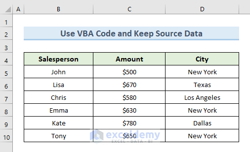
Case 4.1 – Keep Source Data and Copy Rows Automatically to Another Sheet in Excel
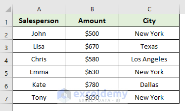
We will copy the rows from the dataset given below.
Steps:
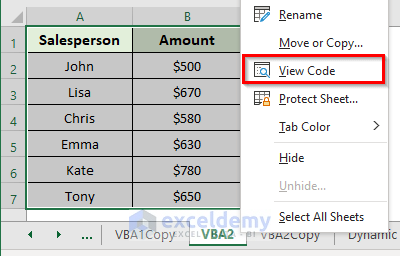
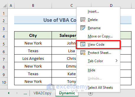
- Right-click on the sheet name from which you want to copy rows. Select the option “View Code”.
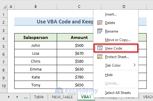
- A new blank VBA module will appear.
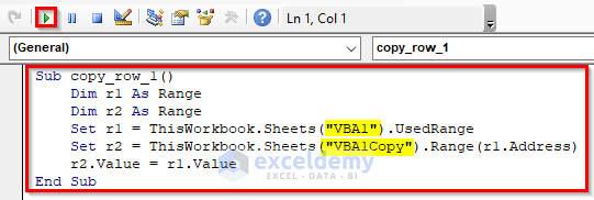
- Insert the following code in the blank window:
Sub copy_row_1()
Dim r1 As Range
Dim r2 As Range
Set r1 = ThisWorkbook.Sheets("VBA1").UsedRange
Set r2 = ThisWorkbook.Sheets("VBA1Copy").Range(r1.Address)
r2.Value = r1.Value
End Sub- Click on Run.
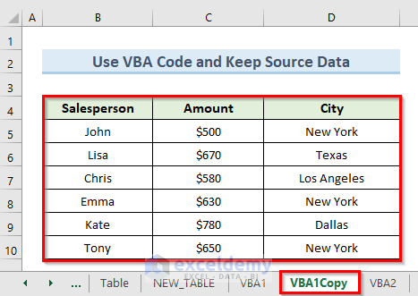
- This code will copy the rows from sheet “VBA1” to “VBA1Copy”. The sheet names are highlighted in the screenshot.
- Go to the sheet “VBA1Copy”. All of the rows from sheet “VBA1” are copied. If you go back to sheet “VBA1”, the source data is unchanged.
Case 4.2 – Automatically Copy Rows to Another Sheet and Remove from Source Data in Excel
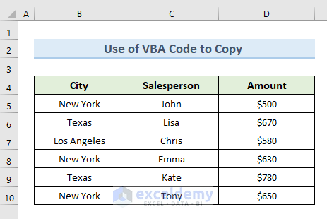
We will copy only the rows in the dataset below that have the value “New York” in the column City and remove it from the dataset.
Steps:
- Select the data range (A1:C7).
- Right-click on the worksheet name.
- Click on View Code.
- You’ll get a blank VBA.
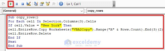
- Insert the following code in the window:
Sub copy_rows()
For Each cell In Selection.Columns(3).Cells
If cell.Value = "New York" Then
cell.EntireRow.Copy Worksheets("VBA2Copy").Range("A" & Rows.Count).End(3)(2)
cell.EntireRow.Delete
End If
Next
End Sub- Click on Run.
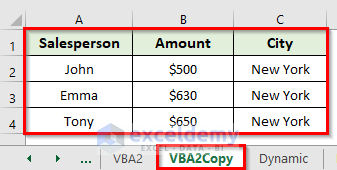
- This code will copy the rows from sheet “VBA2” to “VBA2Copy”.The sheet names are highlighted in the screenshot.
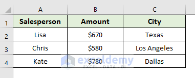
- This deletes the row from the sheet “VBA2” that has the value “New York” in the column City.
- If you go to sheet “VBA2Copy”, all the rows with the value “New York” in column City are moved in that sheet.
Case 4.3 Copy Rows in Excel to Another Sheet Dynamically
This time, the code will group the values of column City by their name. Then, it will copy the values with the same name to an individual worksheet.
Steps:
- Select the sheet Dynamic.
- Right-click on the sheet name and select the option “View Code”.
- You’ll get a new blank VBA.
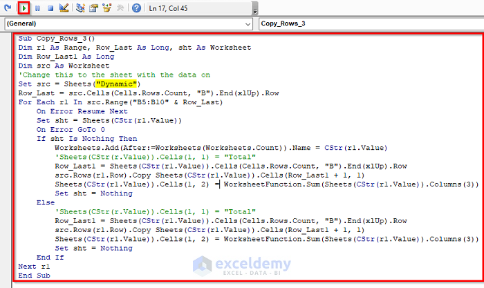
- Insert the following code in the window:
Sub Copy_Rows_3()
Dim r1 As Range, Row_Last As Long, sht As Worksheet
Dim Row_Last1 As Long
Dim src As Worksheet
'Change this to the sheet with the data on
Set src = Sheets("Dynamic")
Row_Last = src.Cells(Cells.Rows.Count, "B").End(xlUp).Row
For Each r1 In src.Range("B5:B10" & Row_Last)
On Error Resume Next
Set sht = Sheets(CStr(r1.Value))
On Error GoTo 0
If sht Is Nothing Then
Worksheets.Add(After:=Worksheets(Worksheets.Count)).Name = CStr(r1.Value)
'Sheets(CStr(r.Value)).Cells(1, 1) = "Total"
Row_Last1 = Sheets(CStr(r1.Value)).Cells(Cells.Rows.Count, "B").End(xlUp).Row
src.Rows(r1.Row).Copy Sheets(CStr(r1.Value)).Cells(Row_Last1 + 1, 1)
Sheets(CStr(r1.Value)).Cells(1, 2) = WorksheetFunction.Sum(Sheets(CStr(r1.Value)).Columns(3))
Set sht = Nothing
Else
'Sheets(CStr(r.Value)).Cells(1, 1) = "Total"
Row_Last1 = Sheets(CStr(r1.Value)).Cells(Cells.Rows.Count, "B").End(xlUp).Row
src.Rows(r1.Row).Copy Sheets(CStr(r1.Value)).Cells(Row_Last1 + 1, 1)
Sheets(CStr(r1.Value)).Cells(1, 2) = WorksheetFunction.Sum(Sheets(CStr(r1.Value)).Columns(3))
Set sht = Nothing
End If
Next r1
End Sub- Click on Run.
- This code will copy the rows from sheet “Dynamic” to individual sheets. The individual sheet is named after the values of column City.
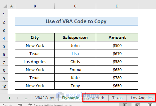
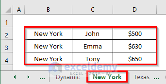
- If you click on sheet “New York”, only the rows that have the value “New York” are in this sheet.
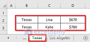
- Cick on sheet “Texas”, and you’ll get only the rows that have the value “Texas” in this sheet.
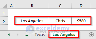
- Click on sheet “Los Angeles” to get rows that have the value “Los Angeles” in the sheet.
Read More: Copy Rows from One Sheet to Another Based on Criteria
Download the Practice Workbook
Related Articles
- Copy Every Nth Row in Excel
- Copy Alternate Rows in Excel
- Copy Rows in Excel with Filter
- Copy Excluding Hidden Rows in Excel
<< Go Back to Copy Rows | Copy Paste in Excel | Learn Excel
Get FREE Advanced Excel Exercises with Solutions!

Is there a way to do this for multiple values to go to a different tab?
Example: I have a list of employees with different types of employment; Federal, Casual Hire, Contract, Forest Service, etc.
I have my main sheet (Master), I have column E that classifies which type of employee they are, I want that row to copy to a new tab depending on which group they are in.
In other words, I would like a tab for Federal with all the federal from column E to copy into it, a tab for casual hire with all the casual hire from column E, etc.
Thank you for any help you can give
Hello DESTINY,
First, thanks for your curious question. It was amusing to solve the problem. Let me guide you to fulfill your query.
Step 1. Assume you have a Dataset where you have the Names of the employees in one column and the types of the employees in another.
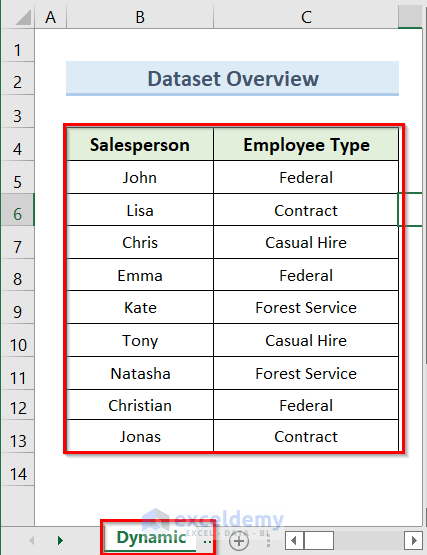
Step 2. Then insert the following code in the VBA window.
Sub Copy_Rows_3()
Dim r1 As Range, Row_Last As Long, sht As Worksheet
Dim Row_Last1 As Long
Dim src As Worksheet
‘Change this to the sheet with the data on
Set src = Sheets(“Dynamic”)
Row_Last = src.Cells(Cells.Rows.Count, “C”).End(xlUp).Row
For Each r1 In src.Range(“C5:C13” & Row_Last)
On Error Resume Next
Set sht = Sheets(CStr(r1.Value))
On Error GoTo 0
If sht Is Nothing Then
Worksheets.Add(After:=Worksheets(Worksheets.Count)).Name = CStr(r1.Value)
‘Sheets(CStr(r.Value)).Cells(1, 1) = “Total”
Row_Last1 = Sheets(CStr(r1.Value)).Cells(Cells.Rows.Count, “B”).End(xlUp).Row
src.Rows(r1.Row).Copy Sheets(CStr(r1.Value)).Cells(Row_Last1 + 1, 1)
Sheets(CStr(r1.Value)).Cells(1, 2) = WorksheetFunction.Sum(Sheets(CStr(r1.Value)).Columns(3))
Set sht = Nothing
Else
‘Sheets(CStr(r.Value)).Cells(1, 1) = “Total”
Row_Last1 = Sheets(CStr(r1.Value)).Cells(Cells.Rows.Count, “B”).End(xlUp).Row
src.Rows(r1.Row).Copy Sheets(CStr(r1.Value)).Cells(Row_Last1 + 1, 1)
Sheets(CStr(r1.Value)).Cells(1, 2) = WorksheetFunction.Sum(Sheets(CStr(r1.Value)).Columns(3))
Set sht = Nothing
End If
Next r1
End Sub
N.B. if you are following our article, use the VBA code under the method “Copy Rows in Excel to Another Sheet Dynamically” and change the marked portions.
Step 3. After pressing Run, you will get the result in individual desired cells.
Thanks
Good morning,
I am trying to update an existing excel file to make it a bit more efficient. At this point I am having to copy, paste and assort data from an Access file. I am looking to take the data from the Access file, place a copy of it on the source sheet, and then have excel automatically put a copy of each row on their appropriate sheets based on the plant listed on column “L”.
I have downloaded the example excel file and attempted the example/instructions you give in 4.2. However, when I try this on either my excel or yours I get the errors code ‘1004’
If you have any idea what is causing this and it’s solution, I would sincerely appreciate your help. Thanks
Hello MICHAEL,
Thanks for the amazing question. Let me guide you in solving this problem.
If you want to solve this problem at first you have to know the possible reason behind this problem.
The first reason can be MACRO NAME ERROR.
This problem occurs if VBA code is used but the file has not been saved as ‘Macro-Enabled Workbook’.
The second reason can be FILE CONFLICT.
This problem occurs when the file has many codes and somehow they get conflicted with each other.
Another reason can be “TOO MUCH LEGEND ENTRIES”
If the excel chart has more legend entries than the space available then this problem occurs.
The last possible reason can be “EXCEL FILE CORRUPTION”
In this case, the whole file got corrupted or damaged, or infected.
Though many reasons can cause this error 1004 problem luckily we can fix it with the help of some easy methods.
Solution 1. Deleting GWXL97.XLA Files
Step 1. Go to C:\Program Files\MS Office\Office\XLSTART.
Step 2. Find GWXL97.XLA file and delete it.
Step 3. After deleting the file, reopen the excel file and check if the problem is solved or not.
Solution 2. Check Trust Access
Step 1. Open the excel file.
Step 2. Click on the Files option and press Option.
Step 3. Go to the ‘Trust Center Option’ and enter into the ‘Trust Center Settings’ option.
Step 4. After that go to the ‘Developer Macro Settings’ and click the tick option and check if the problem is solved or not.
Solution 3. Create Another ‘Macro-Enabled Workbook Template’
Step 1. Open a new workbook and entry the data as before.
Step 2. Go to File>Save As options.
Step 3. In the File name section, select the Excel Macro-Enabled Workbook option.
Step 4. Save the file with the desired name.
These solutions should solve your problem. If you face any further problems, please let us know so that we can help you. Thanks.
Hi Rian,
I am able to run the code but it is only fetching first row and created sheet but not populating the second row. its giving run time error 1004
Hey Bharat, thanks for reaching out. Could you specify the code that face problem using it?
I have more complicated situation. I’m not sure it’s even possible to do but maybe you can help me. I have 1 Sheet full of data and 2 sheet full of data. I want to merge these sheets, so transfer data from one sheet to another. But the transfer should happened into the specific rows. For example:
Data from Sheet 1 (A10072:AT10801) has to go to Sheet 2 (A10772:AT10801) and data from Sheet 1 (A10802:AT10831) has to go to Sheet 2 (A10802:AT10831). Simple formula and clicking and dragging would not work as its too much time wasted. Maybe you have a solution for me
Hello JUSTINA!
I have an easy solution to your problem. To copy data of range Sheet1 (A10072:AT10801) to range Sheet 2 (A10772:AT10801), you can use this VBA Code.
And to copy data of range Sheet 1 (A10802:AT10831) to the range Sheet 2 (A10802:AT10831), use the following VBA code-
I hope, your problem will be solved in this way. You can share more problems in an email at [email protected]
Hello!
I was successful in using your instructions here- 4.3 Copy Rows in Excel to Another Sheet Dynamically to have my data filter to In-Progress or Complete tabs. Two problems and/or questions you may be able to assist with.
1. Is there anyway to make this process not duplicate data which has already copied over. For example. If I add a row of data to the dynamic tab and run the process it copies overall all the data not just the new data added.
2. I was trying to also add separate code or logic to the In Progress tab that if Column M changes to complete it would delete it from this tab and move it to the Complete tab. I can’t seem to get this to work even when using your notes here 4.2 Automatically Copy Rows to Another Sheet and Remove from Source Data in Excel. I am not getting an error message, simply nothing happens.
Any help to these 2 issues would be greatly appreciated!
Hello CALEY FORBES,
Thanks for the amazing question. Let me guide you in solving this problem.
First, I want to solve your first query. I think to solve your problem it is better to use our first method ‘Automatically Copy Rows in Excel to Another Sheet Using Filters’ method than using VBA code. The reason behind this is I think the first method will do your desired work without hesitation.
For the second query, you have to insert the following formula in the VBA windows.
Sub Cut_Range_To_Clipboard()
Range(“B4:B10”).Cut ‘This will cut the source range and copy the Range “B4:B10” data into Clipboard
‘Now you can select any range and paste there
Range(“J2”).Select
ActiveSheet.Paste
End Sub
Note: in the Range section you can change the desired option to paste accordingly.
I hope, your problem will be solved in this way. You can share more problems in an email at [email protected]
Happy Excelling!!!
Hello,
I have tried to use the code for Copying Rows in Excel to Another Sheet Dynamically and it is working well except that it creates a blank sheet and getting an error code 400. Are there other variables/ranges that I need to adjust?
Regards,
Hello again,
Just to add to my question, I am getting an error on the line below.
Worksheets.Add(After:=Worksheets(Worksheets.Count)).Name = CStr(r1.Value)
Regards,
Thanks XAVIER for your correction.
Actually, there is just a little mistake in the code. Instead of writing B5:B, it’s been written B5:B10. This correction has worked perfectly for me.
You can submit more problems to us at [email protected]. Regards!
Is there a way to make this code only copy values and not formulas?
For Each cell In Selection.Columns(3).Cells
If cell.Value = “New York” Then
cell.EntireRow.Copy Worksheets(“VBA2Copy”).Range(“A” & Rows.Count).End(3)(2)
End If
Next
End Sub
Hello, Rick!
Thanks for sharing your problem with us!
While copying, you have to copy the whole thing (values + formulas). You can have the values (without any formula) only while pasting the copied portion into another place.
While pasting, instead of using ‘.Paste‘ to replicate a formula result as a value rather than the formula itself, use ‘.PasteSpecial‘.
Hope this will help you!
Good Luck!
Regards,
Sabrina Ayon
Author, ExcelDemy.
instead of selection i want to define cell range like a1 to z100 then what will be the sentence
For Each cell In Selection.Columns(3).Cells
If cell.Value = “New York” Then
cell.EntireRow.Copy Worksheets(“VBA2Copy”).Range(“A” & Rows.Count).End(3)(2)
End If
Next
End Sub
Hello DILIP,
Thank you for taking the time to read our article.
In order to automatically copy rows from specific cell ranges without manually selecting them, you will need to include a few lines of code. Here is an example of the code that can be used. Just make sure to adjust the “wsDestination” variable to match the sheet name of your dataset and update the cell ranges in “sourceRange” variable.
We hope this helps! Let us know if you have any further questions.
Regards,
Exceldemy Team
Typo: “Then got to the Data From the drop-down of the “Sort & Filter” option select the option “Filter”.”
Hello Jim Pratt
Thanks for noticing the typo. We have updated the section accordingly.
Regards
ExcelDemy