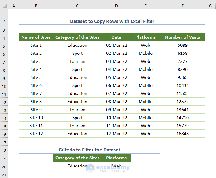
In this article, we will demonstrate 5 ways to copy filtered rows in Excel. We’ll use the dataset below (B1:F16 cell range) to illustrate our methods. 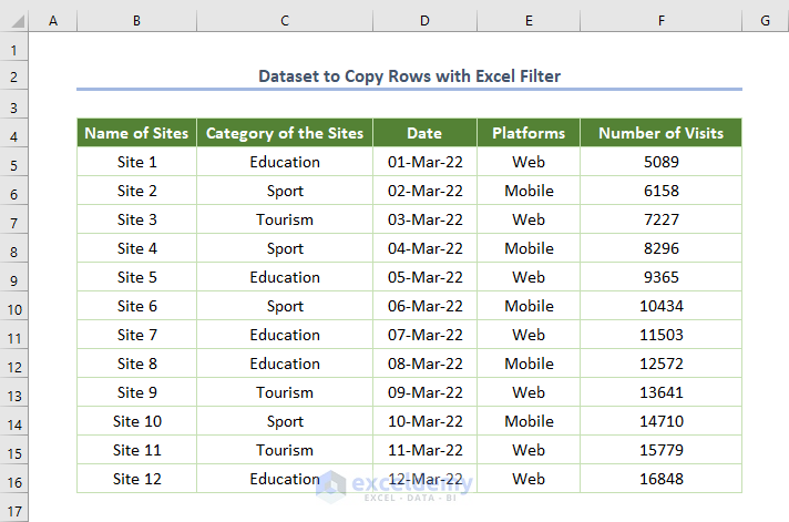
For example, suppose we want to filter the dataset based on Education, which appears in the Category of the Sites column.
Steps:
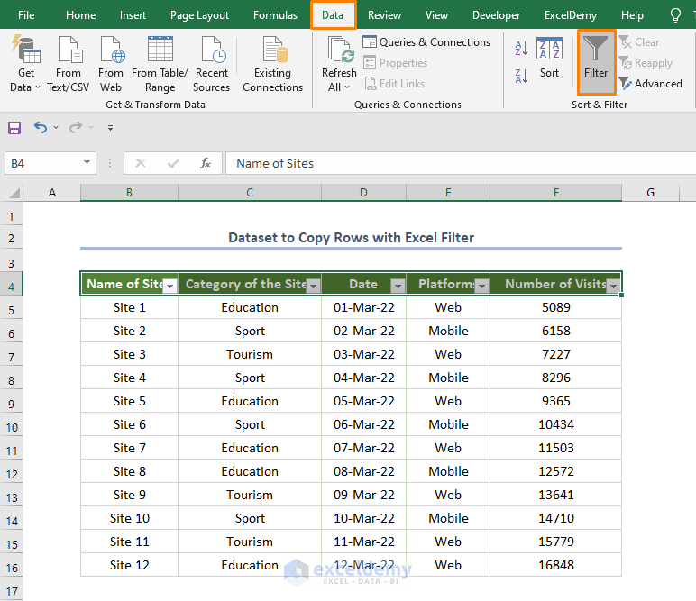
- Select the Filter option from the Data tab.
- Click the filter arrow next to the Category of the Sites column heading.
- Check the box before Education and uncheck the rest of the boxes.
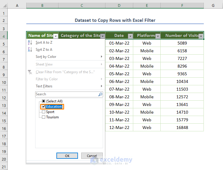
- Click OK.
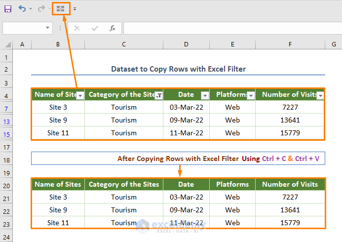
The result is the following filtered rows.
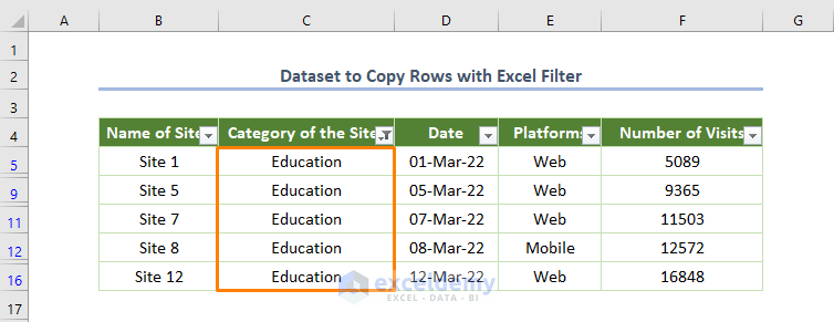
Now let’s see how to copy filtered rows like these quickly in Excel.
Method 1 – Using the Go To Special Option
A simple tool to copy filtered rows is application of the Go To Special option.
Steps:
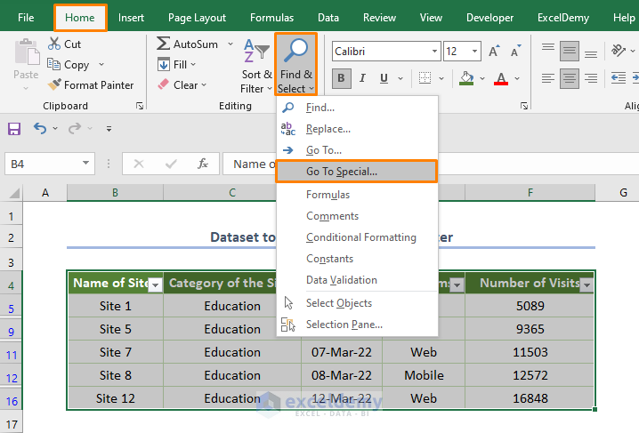
- Select the range of filtered rows (B4:B16).
- Click on the Find & Select option in the Editing section of the Home tab.
- Select Go To Special from the list of options.
- In the Go To Special dialog box that opens, check the circle before the Visible cells only option.
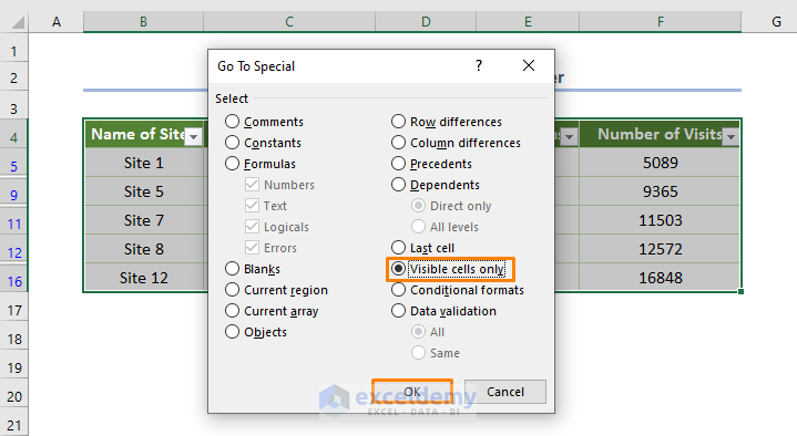
- Press OK,
- Press Ctrl + C to copy the range of filtered rows.
- Paste the filtered data by pressing Ctrl + V.
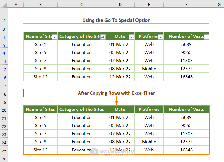
As in the above picture, the filtered data are copied without any hidden rows.
Note: In the above picture, the filtered rows were pasted into the same sheet, however you may accomplish the task in a new sheet in the same manner.
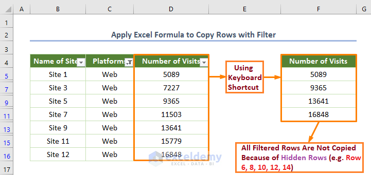
Method 2 – Using the Keyboard Shortcut
You don’t need any option or tool to copy filtered rows if you know the shortcuts.
Steps:
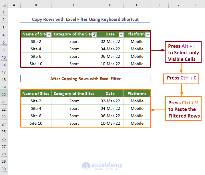
- Select the filtered rows.
- Press Alt + ; to select the visible cells only.
- Press Ctrl + C to copy the visible cells.
- Press Ctrl + V to paste them in a new destination.
The result is like the following screenshot.
Note: When the filter is clear, copy the filtered rows simply by pressing Ctrl + C to copy and Ctrl + V to paste. In other words, there’s no need to press Alt + ;.
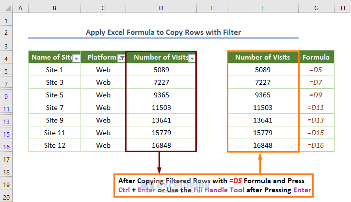
Method 3 – Using an Excel Formula
In the first image below there is an unexpected issue.
Looking at Column F, all filtered rows of Column D haven’t been copied exactly. The reason is that there are hidden rows.
To resolve the issue:
- Insert the following formula in cell F5:
=D5
Here, D5 is the starting cell of the Number of Visits.
- Press Ctrl + Enter (or use the Fill Handle tool after pressing the Enter button).
All the filtered rows of Column D are returned.
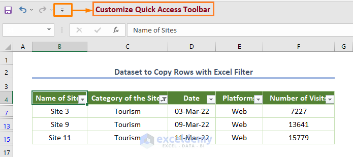
Method 4 – Using a Command from the Quick Access Toolbar (QAT)
The Quick Access Toolbar can be customized to copy filtered rows.
Steps:
- Click on the toolbar.
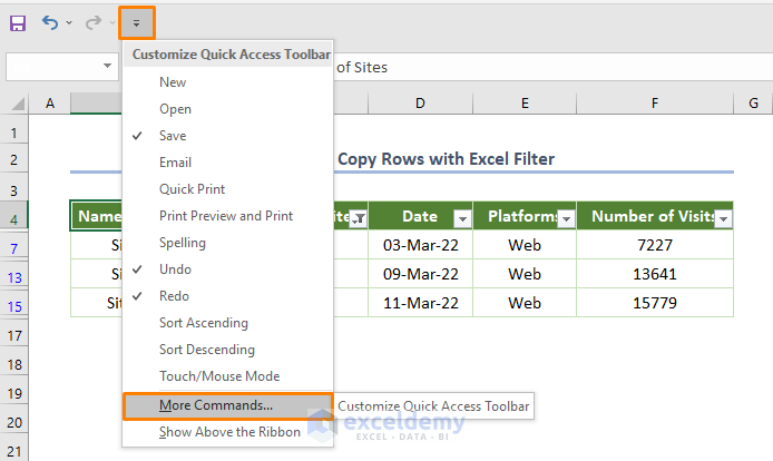
- Click on More Commands.
In the dialog box that opens, select as follows: All Commands > Select Visible Cells > Add > OK.

The Select Visible Cells command now appears in the Quick Access Toolbar.
- Click on the command, then press Ctrl + C and use Ctrl + V to paste the data in a new destination.
Read More: Copy Rows from One Sheet to Another Based on Criteria
Method 5 – Copying Filtered Rows to a New Worksheet Automatically
In the above-discussed methods, to paste into a new worksheet, that worksheet would have to be opened manually. We can open the new worksheet automatically with the filtered rows, using the Advanced Filter tool.
Steps:
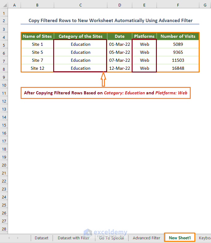
Suppose we want to filter the dataset for either the Education category or Web platform.
- Enter the criteria range in the C19:D20 range as in the image below.
- Make sure that your active sheet is the new working sheet (e.g. New Sheet1 is the new working sheet in the practice workbook).
- Turn on the Advanced filter from the Sort & Filter ribbon in the Home tab,
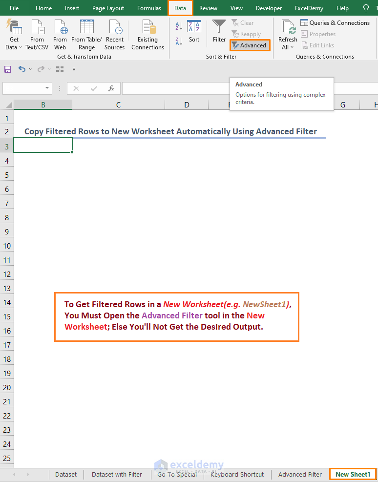
A dialog box named Advanced Filter opens.
- Check the circle before the Copy to another location option.
- Set ‘Advanced Filter’!$B$4:$F$16 as the List range (here, the name of the existing worksheet is Advanced Filter).
- Specify ‘Advanced Filter’!Criteria as the Criteria range.
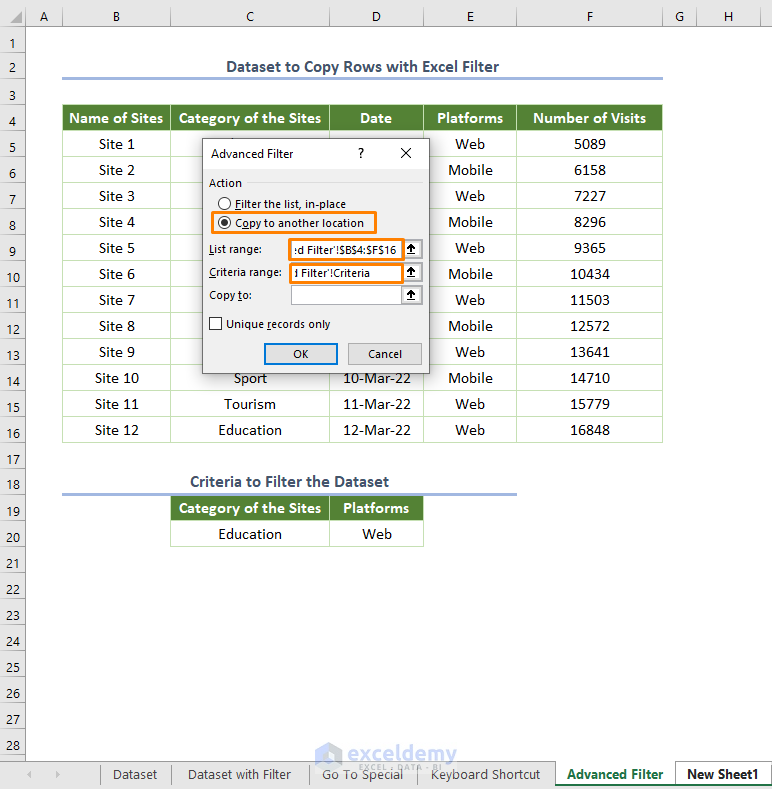
- Set the location ‘New Sheet1’!$B$4:$F$4 in the Copy to box.
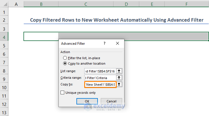
- Click OK.
The filtered rows appear in the new working sheet (New Sheet1).
Read More: Copy Every Nth Row in Excel
Method 6 – Using VBA Code to Copy Rows into a New Sheet
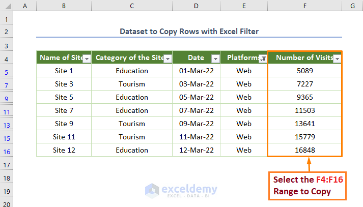
Suppose we want to copy the Number of Visits located in the F4:F16 range.
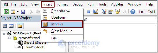
Step 1 – Inserting a Module
- Go to Developer > Visual Basic.
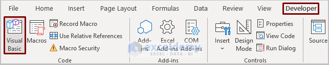
- Go to Insert > Module.
Step 2 – Copying the VBA Code
- Copy the following code and paste it into the newly created module:
Sub Copy_FilteredRows_NewSheet()
Dim Rng As Range
Dim Selecting_FilteredRows As Range
Dim destination As Range
Dim source As Range
Dim r As Range
Set Rng = Application.Selection
Rng.SpecialCells(xlCellTypeVisible).Select
Set Selecting_FilteredRows = Application.Selection
Set destination = Application.InputBox("Please Select the Output Range:", Type:=8)
For Each source In Selecting_FilteredRows
source.Copy
For Each r In destination
If r.EntireRow.RowHeight <> 0 Then
r.PasteSpecial
Set destination = r.Offset(1).Resize(destination.Rows.Count)
Exit For
End If
Next r
Next source
End Sub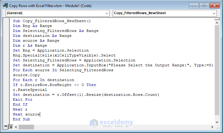
In the above code,
i. We declare some variables: Rng, Selecting_FilteredRows, etc.
ii. We use the Selection property to return the objects to the active sheet.
iii. We use SpecialCells to specify the cells and fix xlCellTypeVisible as the cell type (the first argument) of Special Cells.
iv. We use the Selection property to select the Select_FilteredRows.
v. We set an InputBox to select the output range.
vi. We employ a For Loop to copy the selected filtered rows.
vii. We use an If logical statement to get the value for skipping hidden rows.
viii. Lastly, Offset is used to return a specified input range, and the Resized property is applied to get the resized output.
Step 3 – Running the VBA Code
- Run the code by pressing the keyboard shortcut F5 or Fn + F5).
A dialog box opens requesting the output range.
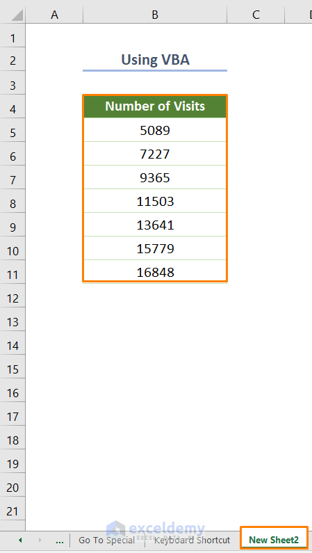
- Select the output range to which to copy the rows. Here, we set ‘New Sheet2’!$B$4:$B$11 as the output range (New Sheet2 is the name of the new working sheet).
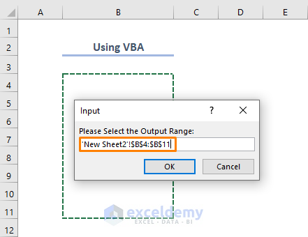
- Click OK after selecting the output range.
The filtered rows are copied to the new sheet.
Download Practice Workbook
Related Articles
- Copy and Paste Thousands of Rows in Excel
- Copy Alternate Rows in Excel
- Copy Excluding Hidden Rows in Excel
- Copy Rows Automatically in Excel to Another Sheet
<< Go Back to Copy Rows | Copy Paste in Excel | Learn Excel
Get FREE Advanced Excel Exercises with Solutions!
