How to Build an Amortization Schedule in Excel

Photo by Jakub Żerdzicki on Unsplash
 

An amortization schedule shows how each loan payment is divided between principal and interest. It also tracks how the outstanding loan balance decreases over time. Excel makes it easy to build a complete amortization schedule using the PMT function and a few simple formulas. This is essential for mortgages, car loans, and any fixed-rate installment loan.

In this tutorial, we will show the steps to build an amortization schedule in Excel. Let’s build a 5-year loan amortization schedule with monthly payments.

Step 1: Set Up Your Input Cells

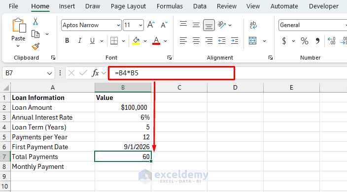
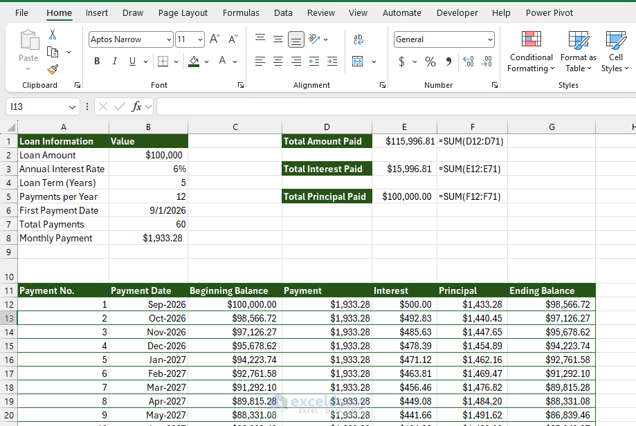
Start with a clean input section at the top of your worksheet; this makes the schedule dynamic, so changing any variable instantly recalculates the whole table.

Calculate the Total Number of Payments:

Since the loan term is 5 years and payments are made monthly, calculate the total number of payments.

• Select cell B7 and enter:

=B4*B5

Step 2: Calculate the Monthly Loan Payment with PMT

Excel’s PMT function calculates the fixed payment required to repay a loan.

• In cell B8, enter the following formula:
• Format Monthly Payment as Currency

=-PMT(B3/B5,B7,B2)

The minus sign before PMT converts Excel’s negative cash-flow result into a positive payment amount. Here:

• B3/B5 converts the annual interest rate into a monthly rate
• B7 represents the total number of payments
• B2 is the original loan amount
• The minus sign before PMT displays the payment as a positive value

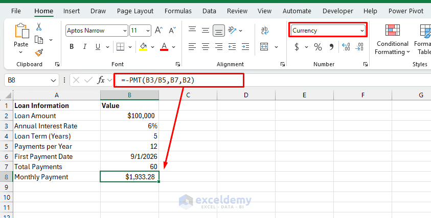
The payment stays the same every month for a standard fixed-rate loan.

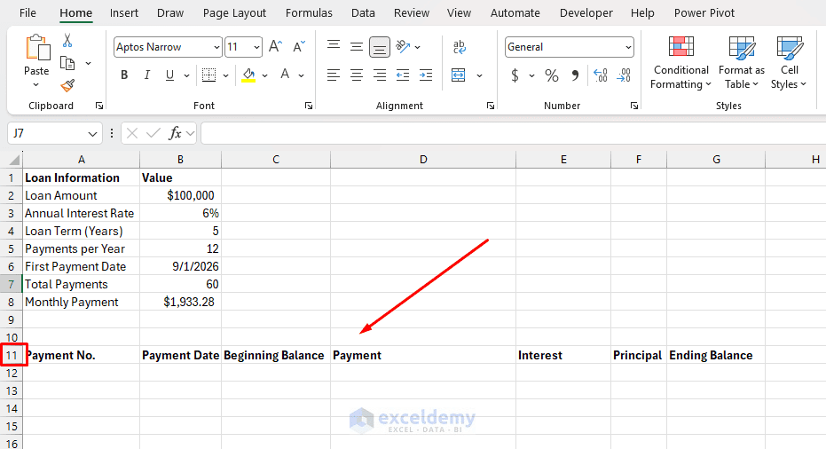
Step 3: Create the Amortization Schedule Headers

• Starting in row 11, create the following columns:

Step 4: Populate the First Row of the Schedule

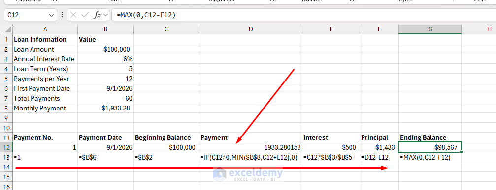
First Payment Number:

• In the Payment No. column, cell A12, enter the first payment number:

=1

You now have one row for each monthly payment.

Payment Date:

• In the Payment Date column, cell B12, reference the first payment date:

=$B$6

This makes the first row of the schedule correspond to the first loan payment.

Enter the Beginning Loan Balance:

The beginning balance for the first payment is simply the original loan amount.

• In cell C12, enter:

=$B$2

The $ symbols create an absolute reference, so Excel always refers to the original loan amount.

Calculate the Interest Portion:

Interest for each payment period is calculated from the outstanding loan balance.

• In cell E12, enter:

=C12*$B$3/$B$5

This multiplies the beginning balance by the monthly interest rate. For the first payment:

Interest = $100,000 × 6% ÷ 12 = $500

Therefore, $500 of the first payment goes toward interest.

Calculate the Payment Amount:

• In cell D12, enter:

=IF(C12>0,MIN($B$8,C12+E12),0)

Normally, this returns the fixed monthly payment stored in B8. The MIN function handles the final payment by preventing it from exceeding the remaining loan balance plus interest.

Calculate the Principal Portion:

The amount applied to principal is the total payment minus the interest.

• In cell F12, enter:

=D12-E12

For the first payment, the calculation is approximately $1,433.28. Therefore, about $1,433.28 of the first payment reduces the loan balance.

Calculate the Ending Balance:

Subtract the principal payment from the beginning balance.

• In cell G12, enter:

=MAX(0,C12-F12)

Using MAX prevents Excel from displaying a tiny negative balance caused by rounding. After the first payment, the remaining loan balance will be approximately $98,566.72.

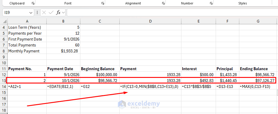
Step 5: Create the Second Payment Row

Now create the formulas for the next payment.

• Payment Number (A13):

=A12+1

• Payment Date (B13):

=EDATE(B12,1)

EDATE moves the payment date forward by one month.

• Beginning Balance (C13):

=G12

The previous payment’s ending balance becomes the next payment’s beginning balance.

• Payment (D13):

=IF(C13>0,MIN($B$8,C13+E13),0)

• Interest (E13):

=C13*$B$3/$B$5

• Principal (F13):

=D13-E13

• Ending Balance (G13):

=MAX(0,C13-F13)

Step 6: Fill the Formulas Down

The sample loan requires 60 monthly payments.

• Select the formulas in A13:G13
• Drag the Fill Handle downward until the schedule contains all 60 payments
• Since the first payment is in row 12, the 60th payment will appear in row 71

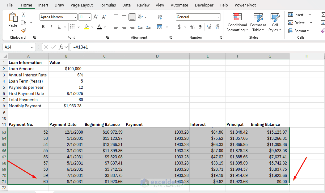
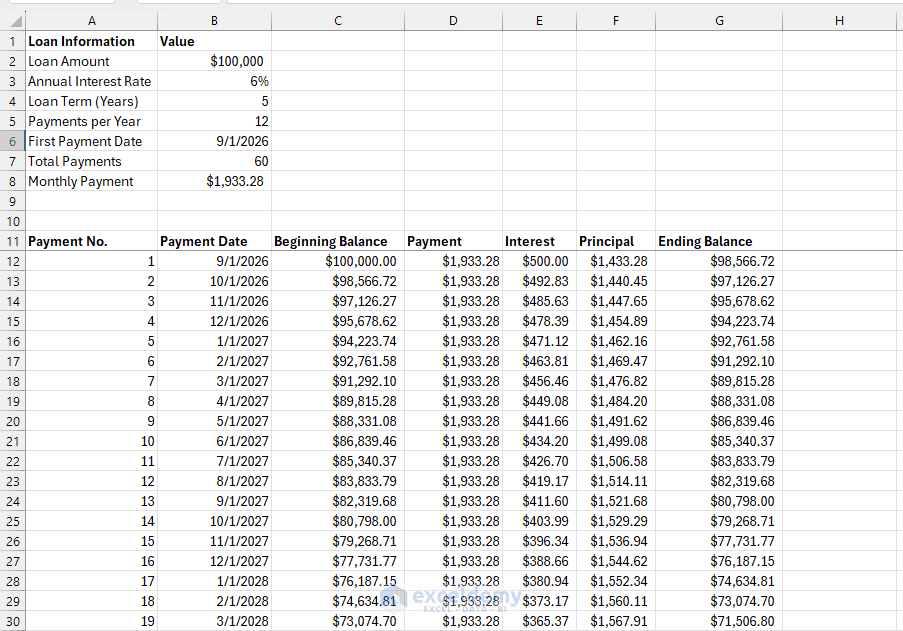
As the schedule progresses, you will notice that:

• Interest decreases
• Principal increases
• The payment remains almost constant
• The loan balance gradually approaches zero

This is the main characteristic of a standard amortizing loan.

Step 7: Calculate Total Payments and Total Interest

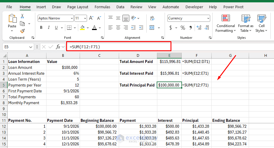
You can add a small summary below the schedule.

• Total Amount Paid

=SUM(D12:D71)

This returns the total amount paid over the life of the loan.

• Total Interest Paid

=SUM(E12:E71)

This shows how much the loan costs in interest.

• Total Principal Paid

=SUM(F12:F71)

The total principal should be approximately equal to the original $100,000 loan amount.

Using IPMT and PPMT Instead

Excel also includes dedicated functions for calculating the interest and principal portions of individual payments.

Calculate Interest with IPMT

Its syntax is:

=IPMT(rate,per,nper,pv)

You can replace the interest formula with:

=-IPMT($B$3/$B$5,A12,$B$7,$B$2)

The IPMT function returns the interest portion of a specific loan payment. Here, A12 identifies the payment period.

Calculate Principal with PPMT

Its syntax is:

=PPMT(rate,per,nper,pv)

Similarly, the principal portion can be calculated with:

=-PPMT($B$3/$B$5,A12,$B$7,$B$2)

Using IPMT and PPMT is particularly useful when you need to retrieve the principal or interest for a specific payment without constructing the entire calculation manually.

Format the Amortization Schedule

For a cleaner worksheet:

• Format Loan Amount, Monthly Payment, Beginning Balance, Payment, Interest, Principal, and Ending Balance as Currency
• Format Annual Interest Rate as Percentage
• Format the Payment Date column as a date, such as mmm-yyyy
• Apply bold formatting to the table headers
• Add borders or convert the range into an Excel Table for easier viewing
• You can freeze the schedule header row for better scrolling

You can also apply conditional formatting to the Ending Balance column to highlight when the loan reaches zero.

Create a Principal vs. Interest Chart

An amortization chart makes it easier to see how the composition of each payment changes.

• Select the Payment No., Interest, and Principal columns from the schedule
• Go to the Insert tab >> select Column or Bar Chart >> select Stacked Column

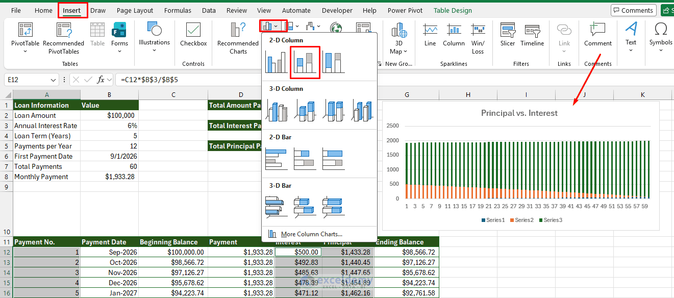
The chart will show that early payments contain more interest, while later payments contain more principal.

Make It Handle Extra Payments (Optional)

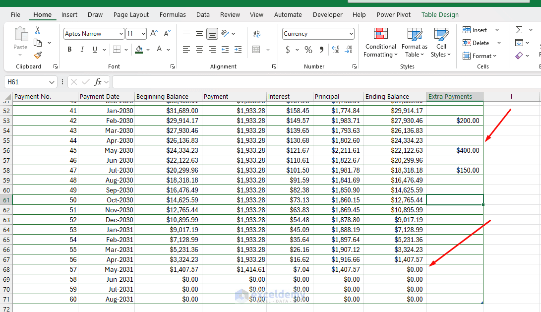
To model extra principal payments, add a column H labeled “Extra Payment,” let the user enter values there, and adjust:

Principal (Now Includes Extra):

=MIN(D12-E12+H12,C12)

Ending Balance:

=MAX(0,C12-F12)

The MIN function prevents the schedule from paying down more principal than remains, which matters once extra payments shorten the loan term. The interest and remaining-balance formulas below the payoff point will naturally return zero once the ending balance reaches zero.

Conclusion

By following the steps above, you can build an amortization schedule in Excel. An Excel amortization schedule provides a clear breakdown of how a loan is repaid over time. The PMT function calculates the regular payment, while simple formulas calculate the interest, principal, and remaining balance for every payment period. Once the schedule is created, you can change the loan amount, interest rate, or loan term, and Excel will automatically recalculate the repayment schedule. This makes the worksheet especially useful for comparing mortgages, car loans, personal loans, and other financing options.