Suppose you are in a situation to add a superscript, a letter written just above the standard line, in your Excel data. But you don’t know how to do that. For your convenience, we will discuss eight methods of how to add superscript in your Excel throughout this article.
How to Add Superscript in Excel (8 Easy Methods)
Let’s assume we have a dataset, namely “Final Exam Report of Ninth Grader.”. You can use any dataset suitable for you.

Here, we have used the Microsoft Excel 365 version; you may use any other version according to your convenience.
1. Using Format Cells Option
To add superscripts in your spreadsheet, Excel provides plenty of methods to serve you. Firstly, we will use the Custom Format Cells option to do the task.
📌 Steps:
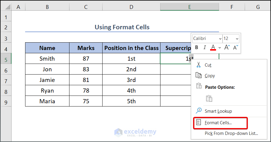
- First, select the text you wish to be superscripted. Here we select “st” as our cell D5 suggests.
- Click on the Right Button of your mouse and then select the Format Cells option.
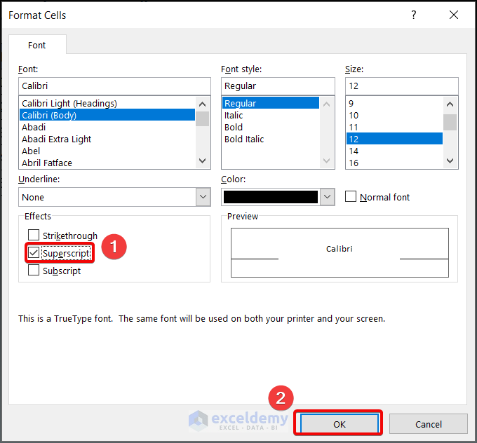
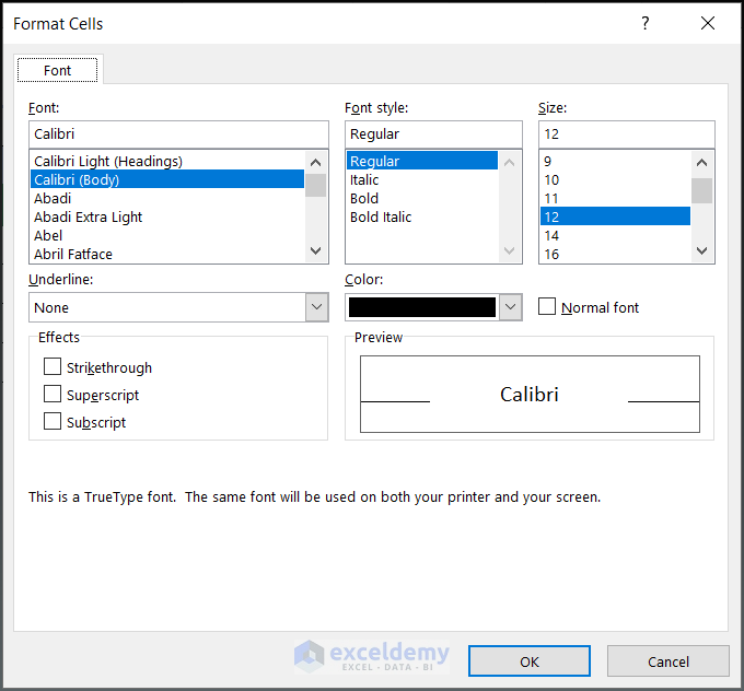
- This will open a dialog box as follows.
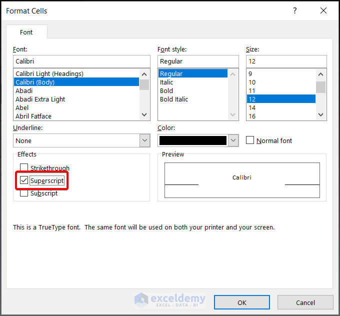
- Check the box before Superscript, then press OK.
- Here is our output as shown below.
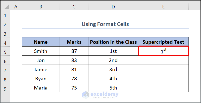
- Now to get the other value, drag the Fill Handle Tool.

Read More: How to Write 1st 2nd 3rd in Excel
2. Utilizing Shortcut Key
The process we described in Method 1 can also be done by using some. That means you don’t have to click on your mouse repeatedly. Just follow the steps we describe below.
📌 Steps:
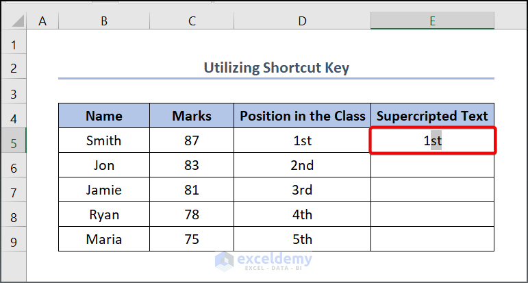
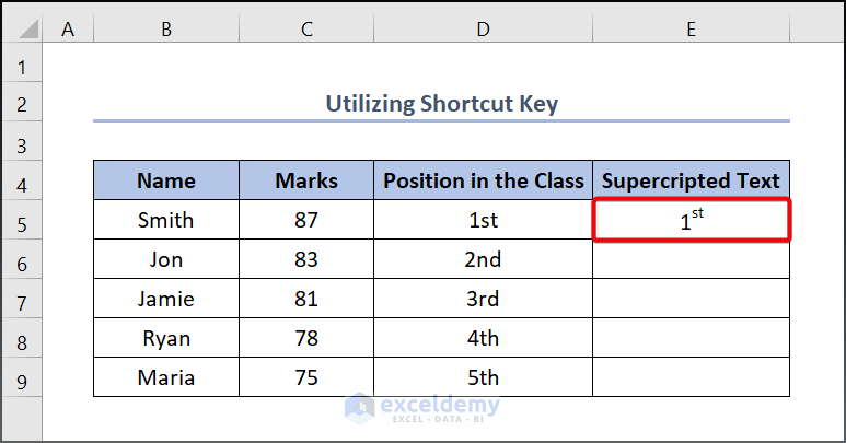
- First, select the intended text that you wish to superscript. Here we select “st” as our cell D5 suggests.
- Now press Ctrl + 1 simultaneously on your keyboard. Thus, the following dialogue box will appear.
- Press Shift + Alt + E afterward.
- Then press the Enter button on your keyboard.
- See the output below. Same as before, isn’t it?
- Drag the Fill Handle tool to get the other value.

3. Adding Superscript Command in Quick Access Toolbar
If you think the abovementioned method can make you slow, then you can add a superscript command to your Quick Access Toolbar. This will make your work easier.
📌 Steps:
- First, click the triangular-shaped icon on the Title Bar and then More Commands.
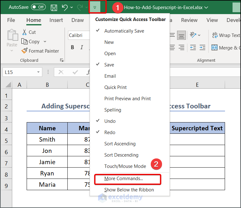
- This will bring a dialog box as below.
- Now scroll down to get more options under Popular Command.
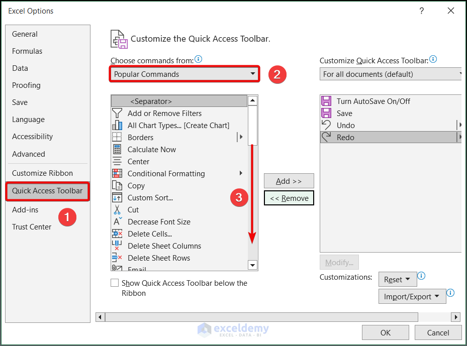
- Select Superscript > Add >> OK.

- Now this will allow you to have a superscript icon in your Title Bar.
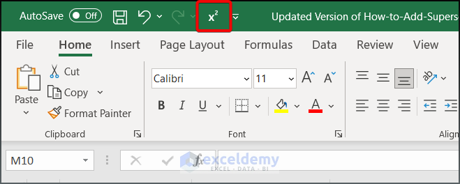
- Now select your intended letters and click on the Superscript (x2) command.

- See the output below.
- As you already understand, once you get the superscript command in your Title Bar, you don’t have to do the process as you do in Method 1 and 2.

- Drag the Fill Handle tool to get the rest of the value.

Read More: [Fixed!] Excel Superscript Not Working
4. Integrating Superscript Option in Excel Ribbon
Another way to do the job is by integrating the superscript option in the Excel Ribbon. See the description below to learn more about it.
📌 Steps:
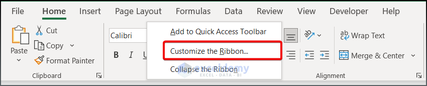
- Click the Right Button on your mouse.
- Now select the Customize the Ribbon option.
- Thus, a dialogue box will appear. Now, follow the process we have demonstrated below.
- Thus, you will get a superscript command in your Ribbon.
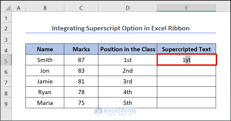
- Now select the text.
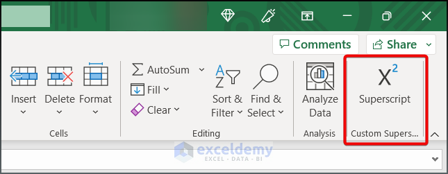
- Then, click on the icon given below.
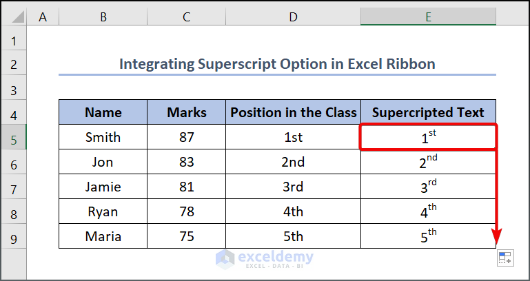
- Here is our output below.

- Drag the Fill Handle tool to get more.
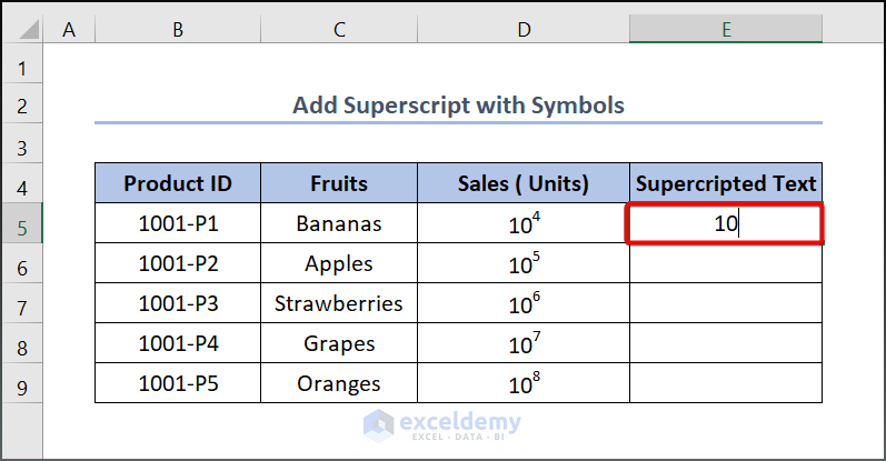
5. Adding Superscript with Symbols
Adding a superscript with a symbol is another way to accomplish the same task. Suppose we have a dataset like the one below, where you have to superscript a number on a number. How will you do that? Well, follow the steps to learn more.

📌 Steps:
- Select the cell where you wish to superscript your number
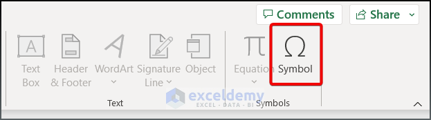
- Click on Insert > Symbol.
- Then select Symbol > Superscripts and Subscripts.

- Now select your superscript symbol in our case which is 4.
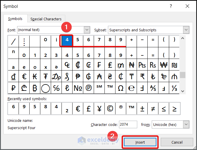
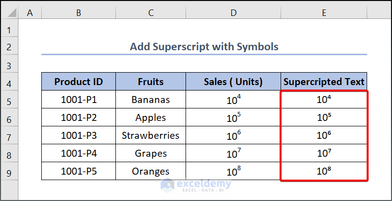
- That’s it. See the image below.

- Get the other value by doing the same process.
Read More: How to Write Subscript in Excel
6. Adding Superscript with the CHAR Function
You can add superscripts by using the CHAR function. Note that, with the CHAR function, it is only possible to return 3 different superscripts (0, 1, and 2).
📌 Steps:
- See the below image to learn the corresponding CHAR code.
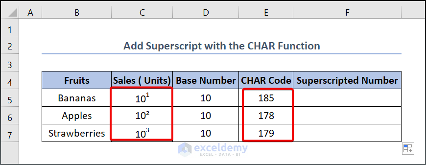
- Now enter the following function in cell F5.
=D5&CHAR(E5)Here, D5 refers to the Base Number and E5 refers to the corresponding CHAR code.
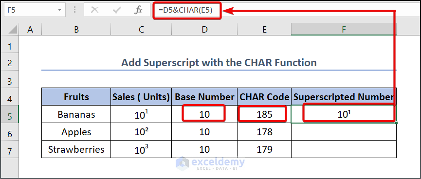
- Drag down the F5 cell to F7 to get the other value.

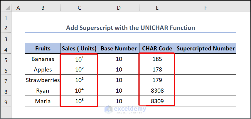
7. Using the UNICHAR Function
As you already understand, there is a limitation to using the CHAR function. However, you can use the UNICHAR function to get your output. In this case, all you need to know is the corresponding UNICHAR code.
📌 Steps:
- The UNICODE can be found in the image below.
- Now enter the following function in cell F5.
=D5&UNICHAR(E5)Here D5 refers to the Base Number and E5 refers to the corresponding UNICHAR code.
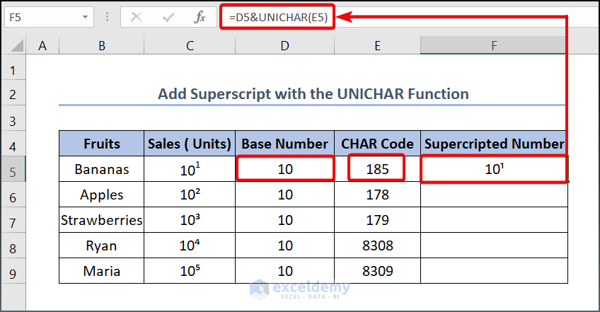
- Drag the Fill Handle to get the second output.

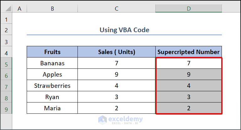
8. Employing VBA Code
Now imagine that you have a long list of data that you need to convert into superscript form. How will you do that? Well, in this situation, the VBA code is for you.
📌 Steps:
- Press Alt + F11 to open your Microsoft Visual Basic.
- Then press Insert > Module to open a blank module.

- Now, write the following VBA code in your Module1.
Sub SuperscriptGenerator()
    Dim SuperscriptRange As Range
    Dim MyCell As Range
    Dim MyString As String
    Dim MyChar As String
    Dim i As Long
    Set SuperscriptRange = Selection
    Application.ScreenUpdating = False
    For Each MyCell In SuperscriptRange
        MyString = MyCell.Value
        For i = 1 To Len(MyString)
            MyChar = Mid(MyString, i, 1)
            If MyChar >= "0" And MyChar <= "9" Then
                MyCell.Characters(i, 1).Font.Superscript = True
            End If
        Next
    Next
    Application.ScreenUpdating = True
End Sub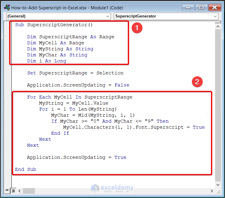
- Close your VBA window.
⚡ Code Breakdown:
Now, we will explain how the given VBA code works. The code is divided into 2 steps.
- In the first portion, there are some variables that we need to use to run the code.
- In the second portion, if your selected data’s range is between 0 to 9 then it will run a loop to give your input data into a superscript form. If your data range is more than 0-9 change the string accordingly.
- Now, choose the range for which you want to turn them into superscripted form.
- Click on Developer > Macros.

- This will open the Macros dialog box. Then select your function, which in this case is SuperscriptGenerator.
- Then, click on the Run

- Now you can see the output as given below.

Things to Remember
- It is worth mentioning that when you superscript any number on another number, don’t forget to add an apostrophe or single quotation (‘) before your number.
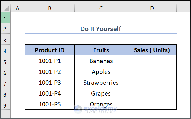
Practice Section
We have provided a Practice section on the right side of each sheet so you can practice yourself. Please make sure to do it yourself.
Download Practice Workbook
Back to Learn Excel > Formatting Text > Subscript and Superscript
Conclusion
I hope you have learned something new today through this tutorial. This is an easy task and I think all of us should learn this method to make our life a little bit easier. Further, If you have any queries, feel free to comment below and I will get back to you soon.
Related Articles
<< Go Back to Subscript and Superscript | Text Formatting | Learn Excel
Get FREE Advanced Excel Exercises with Solutions!
