In Excel, it is a simple task to create an accurate growth formula when all the numbers have a positive value. But there is unfortunately no growth formula with negative numbers in Excel that will return exact, accurate results in all cases. There are different formulas we can use, but misleading or inaccurate results will be returned much of the time. Let’s examine some examples of growth formulas with negative numbers, the issues that arise, and some work-arounds.
The regular formula for the growth rate between any two numbers is:
Growth rate=((New value-Old value)/Old value)*100%.
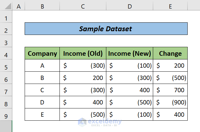
Suppose we have a dataset of 5 different companies and their incomes over two consecutive years.
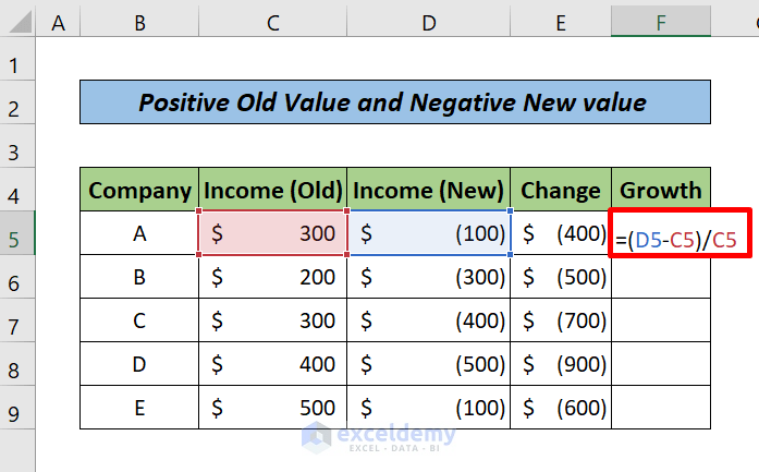
Example 1 – Growth Formula with Positive Old Value and Negative New Value
If only the new values are negative, you can simply apply the regular formula that you use if all values are positive.
Steps:
- Enter the formula below in cell F5:
=(D5-C5)/C5Where:
C5= OId Value (Income the previous year), and
D5= New Value (Income this year)
- Press ENTER to return the growth rate between these two incomes.
- Drag the Fill Handle down to apply the formula to the remaining cells.
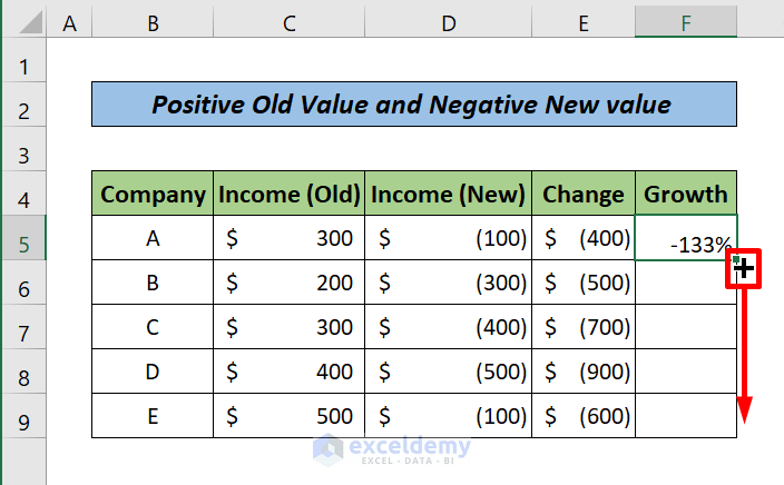
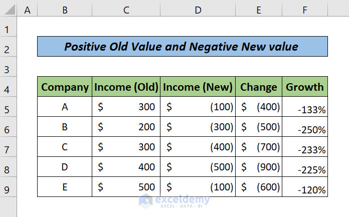
Here is the result:
Note:
Only the new values are negative, meaning they have declined from the old values. Therefore, all the growth results are in negative percentages.
Read More: Growth Over Last Year Formula in Excel
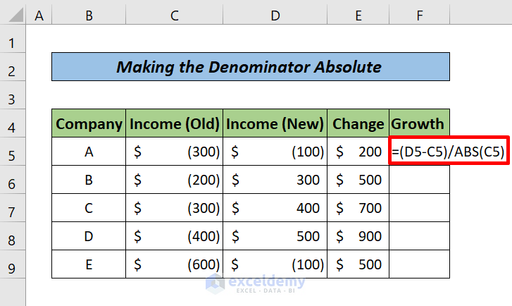
Example 2 – Making the Denominator Absolute
The regular growth formula will not work for the following two cases:
Case 1: When both the values are negative.
Case 2: When the old values are negative and the new values are positive.
For case 2, the formula will always return negative values or losses for the company, while in reality, the movement from negative to positive indicates profits, and so the growth rate should be positive.
For case 1, the same issue will arise, except when absolute new values are smaller than absolute old values.
Making the denominator absolute in our growth formula will partially resolve the issue in both these cases.
- Enter the formula below in cell F5:
=(D5-C5)/ABS(C5)The ABS function returns the absolute or positive denominator value.
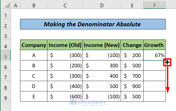
- Press ENTER to return the growth rate between these two incomes.
- Drag the Fill Handle to apply the formula to the remaining cells.
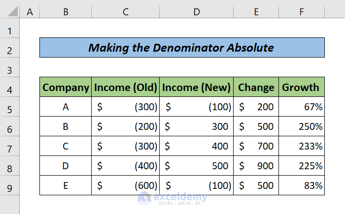
Our growth formula has resolved both case 1 and case 2 issues.
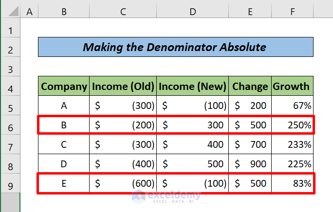
But, there is a complication!
If you look carefully at growth rates for companies B and E, both the growth rates are positive, and the change in the income of E is equal to B. But in reality, E has greater growth or profit than B.
Read More: How to Calculate Year over Year Growth with Formula in Excel
Example 3 – Use IF and MIN Functions to Avoid Misleading Results
The following work-arounds won’t resolve the issue completely, but will prevent the display of inaccurate data.
3.1 No Output for the Negative Numbers
We will search for the negative numbers in both the old and new values. If found, then we will return a text informing that a growth rate cannot be calculated.
Steps:
- Enter the formula below in cell E5:
=IF(MIN(C5,D5)<=0,"Can Not Be Calculated",(D5/C5)-1)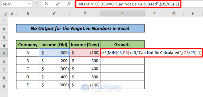
Formula Breakdown:
The IF Function will run a logical test: (MIN(C5,D5)<=0)If the logical test returns TRUE, the function will return the string “Can Not Be Calculated ”. And if the logical test returns FALSE, then the function will return the growth rate between the two values. ((D5/C5)-1)
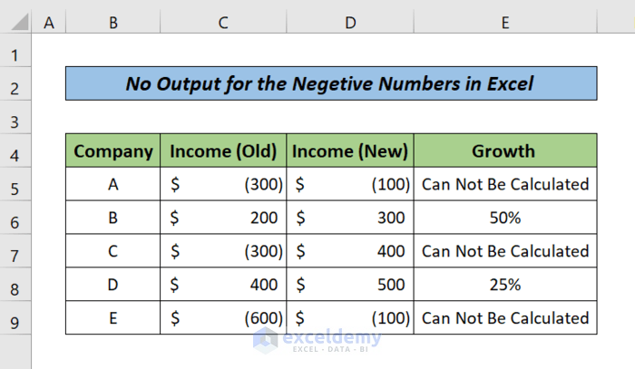
- Press ENTER.
- Drag the Fill Handle to the remaining cells.
Here is the result:
3.2. Show Positive or Negative Growth
Another way is to display “Profit” or “Loss” if there is a negative number and the company produces a profit or a loss.
Steps:
- Enter the following formula in cell F5:
=IF(MIN(C5,D5)<=0,IF((D5-C5)>0,"Profit","Loss"),(D5/C5)-1)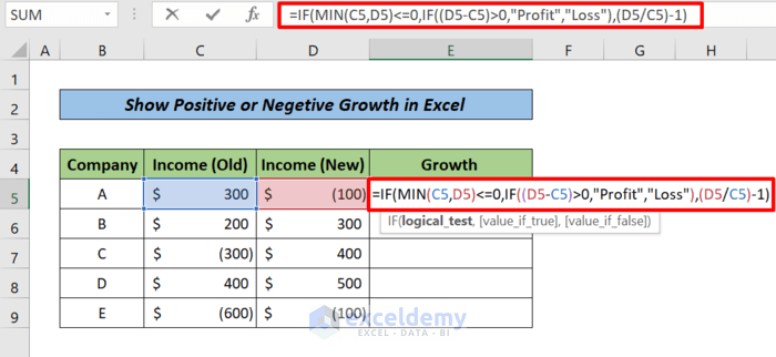
Formula Breakdown:
- The first IF function will run a logical test
(MIN(C5,D5)<=0)to find if there is a negative number in old and new values. If there is a negative number (TRUE), then it will work on the second IF function. - The second IF function runs another logical test
((D5-C5)>0)to find if the new value is greater than the old value. If the new value is greater than the old value (TRUE), then the second IF function will return the string “Profit” (Which indicates positive growth). And if the new value is smaller than the old value (FALSE), then it will return the string “Loss” (Indicates negative growth). - If the logical test in the first IF function returns FALSE, then the function will return the growth rate between the two positive values
((D5/C5)-1).
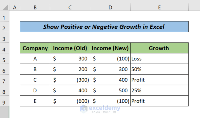
- Press ENTER and drag the Fill Handle to the remaining cells.
Here is the result:
Read More: How to Calculate Growth Percentage with Formula in Excel
Download Practice Workbook
Related Articles
- How to Calculate Annual Growth Rate in Excel
- How to Calculate Dividend Growth Rate in Excel
- How to Use the Exponential Growth Formula in Excel
- How to Calculate Monthly Growth Rate in Excel
- How to Calculate Sales Growth over 3 Years in Excel
- How to Calculate Sales Growth over 5 Years in Excel
- How to Calculate Sales Growth Percentage in Excel
<< Go Back to Growth Formula In Excel | Excel Formulas for Finance | Excel for Finance | Learn Excel
Get FREE Advanced Excel Exercises with Solutions!

Easy to understand and super helpful. Thank you!
Hello Romeo Nyi,
You are most welcome.
Regards
ExcelDemy