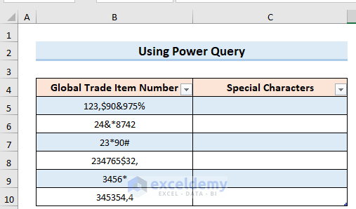
Method 1 – Using the Power Query to Find Special Characters in Excel
Steps:
- This sample table contains Global Trade Item Number in Column B and Special Characters in Column C.
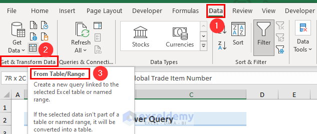
- Go to the Data tab.
- In Get & Transform Data, select From Table/Range.
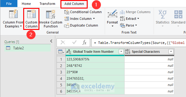
- Table2 will be displayed.
- Go to the Add Column tab and select Custom Column.
- The Custom Column window will open.
- Enter the following formula.
=Text.Remove([Global Trade Item Number],{"A".."z","0".."9"})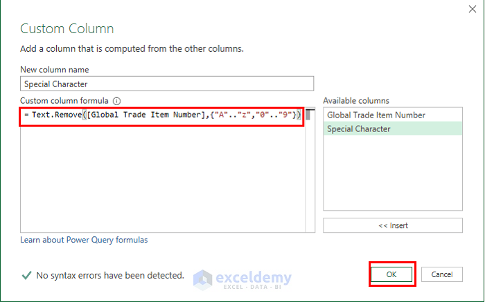
- Click OK to see the result.
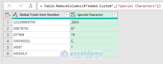
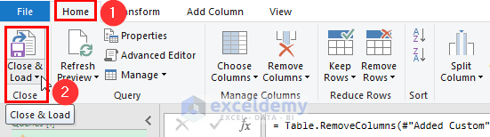
- In the Home tab, select Close & Load.
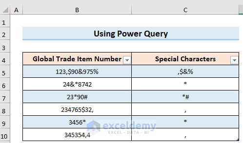
This is the output.
Method 2 – Applying a VBA Code
Steps:
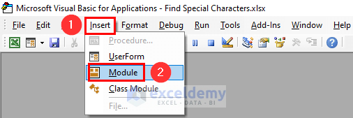
- Press Alt+F11 to open the VBA window.
- In the Insert tab, select Module.
- Enter the following VBA code:
Function FindSpecialCharacters(TextValue As String) As Boolean
Dim Starting_Character As Long
Dim Acceptable_Character As String
For Starting_Character = 1 To Len(TextValue)
Acceptable_Character = Mid(TextValue, Starting_Character, 1)
Select Case Acceptable_Character
Case "0" To "9", "A" To "Z", "a" To "z", " "
FindSpecialCharacters = False
Case Else
FindSpecialCharacters = True
Exit For
End Select
Next
End Function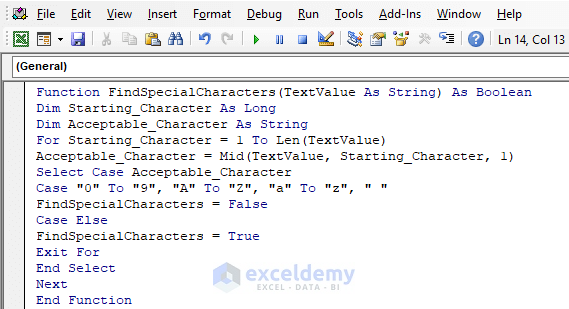
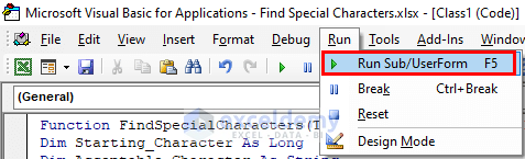
- Click Run or F5.
- Save the code by pressing Ctrl+S.
- Go back to you worksheet, and enter the following formula in C5.
=FindSpecialCharacters(B5)
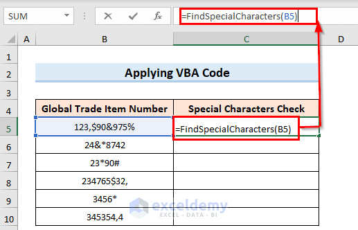
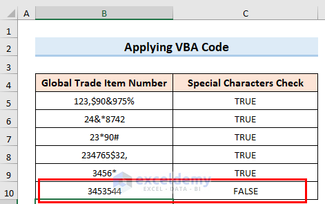
The result for that cell is displayed. As the cell contains special characters, the result is TRUE.
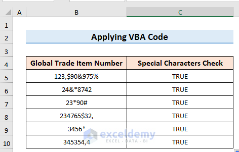
- Use the Fill Handle to Autofill the rest of the cells in the column.

This is the output.
- By changing data with no special characters, FALSE will be displayed.
Method 3 – Applying the User-Defined Function
Steps:
- Follow the steps in Method 2 to open a VBA window. Enter the following code and save it.
Public Function Check_Special_Characters(nTextValue As String) As Boolean
Check_Special_Characters = nTextValue Like "*[!A-Za-z0-9 ]*"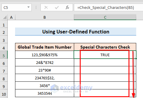
End Function- Enter the following formula in C5.
=Check_Special_Characters(B5)Like in the previous method, TRUE is displayed if the cell contains a special character. Otherwise, FALSE.
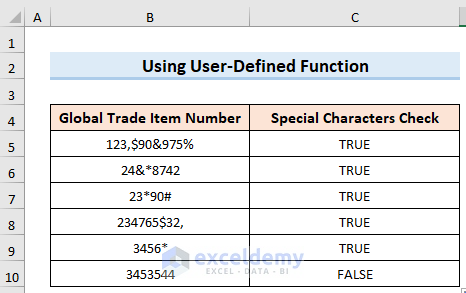
- Use Fill Handle to apply the formula to all cells in the column.
This is the output.
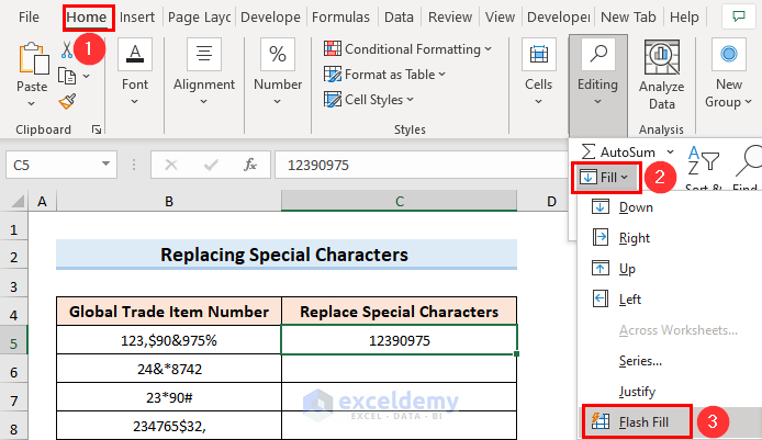
How to Replace Special Characters in Excel
Steps:
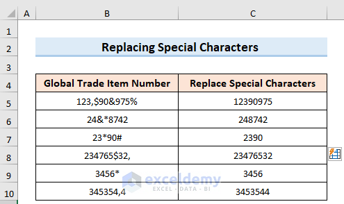
- Enter the data without special characters in C5.
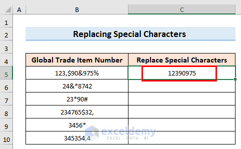
- Go to the Home tab and select Flash Fill from the Fill option.
This is the output.
Download Practice Workbook
Download the practice workbook here.
<< Go Back to Learn Excel
Get FREE Advanced Excel Exercises with Solutions!
