Method 1 – Using Sort & Filter to Calculate Outliers in Excel
Step 1:
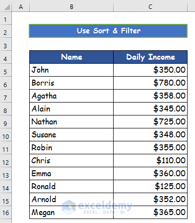
- Select the column header that you want to sort in your Excel dataset. For example, in the given data set, in the file column header named Daily Income (Cell C40 is chosen).
Step 2:
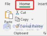
- Press the Home tab on the ribbon and go to the Editing group.
Step 3:
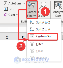
- In the Editing group, click on the Sort & Filter command and click on the Custom Sort.
Step 4:
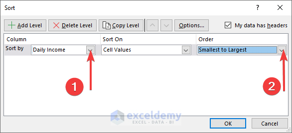
- A new dialog box named Sort will open. In the popped-up dialog box, select Daily Income in the Sort by drop-down and Smallest to Largest in the Order drop-down. Click OK.
Step 5:
- The Daily Income column would be sorted as stated, with the lowest values at the top and the greatest values at the bottom. After running the procedure, look for any irregularities in the data range to determine outliers.
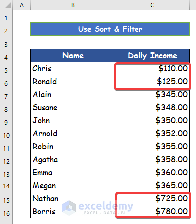
For example, the first two values in the column are significantly lower, and the last two values in the column are substantially higher than the rest of the values in the data set, as shown in the above result.
Read More: How to Find Outliers in Regression Analysis in Excel
Method 2 – Applying the QUARTILE Function to Determine Outliers in Excel
Step 1:
- Enter the following formula for determining the 1st quartile (Q1) given below:
=QUARTILE($C$5:$C$16,1)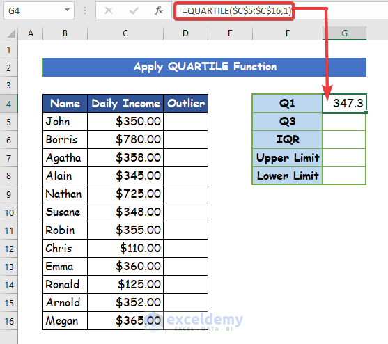
Step 2:
- Enter the formula to calculate the 3rd quartile (Q3) given below:
=QUARTILE($C$5:$C$16,3)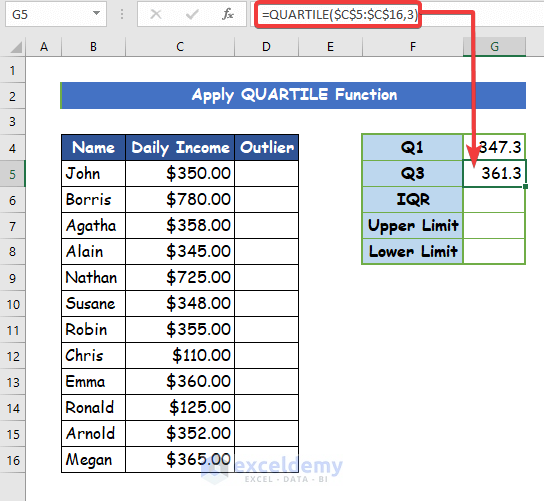
Step 3:
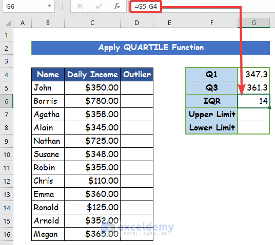
- Determine the IQR, which is the Inter-Quartile Range (it represents 50% of the given data from a range of data sets that fall into the first and third quartiles) by subtracting Q1(in cell G4) from Q3(in cell G5).
- Enter the following formula to calculate the subtraction:
=G5-G4
Step 4:
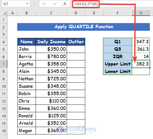
- After finding the IQR, you have to determine the upper and lower limits. The upper and lower limits would contain most of the data within the data set.
- Enter the following formula to calculate the upper limit:
=G5+(1.5*G6)
Step 5:
- Calculate the lower limit. Enter the following formula:
=G4-(1.5*G6)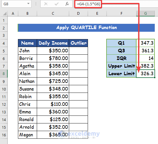
Step 6:
- After finishing the previous step, you can determine outliers for each data value. In the Excel worksheet, enter the following formula with the OR function in cell D5:
=OR(C5<$G$8,C5>$G$7)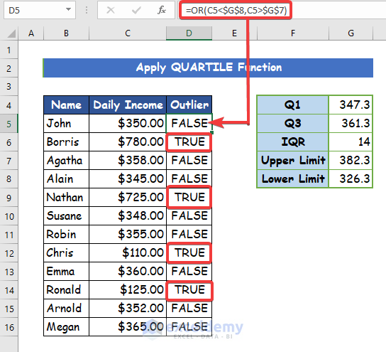
- This formula will help identify the data that do not fall within the range mentioned above limit. After processing, the formula will show a TRUE Statement if the specific data is an outlier and FALSE if it is not. Double-click on the AutoFill tool in cell C5 to copy the formula to the rest of the cells in column C. Thus, you can observe a True value next to all the outliers in your dataset.
Method 3 – Combining AVERAGE and STDEV.P Functions to Calculate Outliers from Mean and Standard Deviation
Step 1:
- Use the same dataset shown at the start of this article and then calculate the mean and standard deviation. To calculate the mean, enter the following formula with the AVERAGE function in cell G5:
=AVERAGE(C5:C16)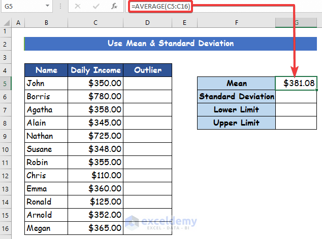
Step 2:
- To calculate the standard deviation, enter the following formula with the STDEV.P function in cell G6:
=STDEV.P(C5:C16)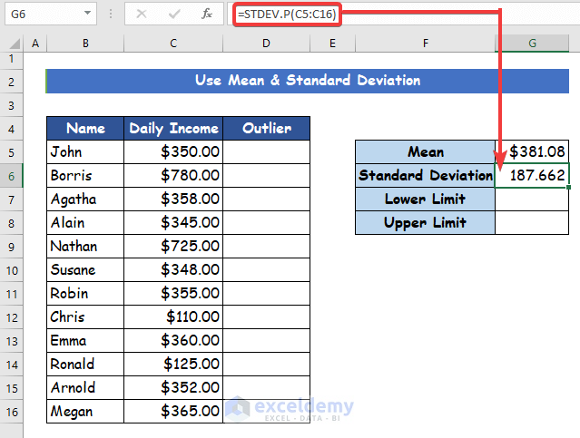
Step 3:
- Calculate the upper limit for further advancement in the process. In cell G7, calculate the lower limit by using the following formula:
=G5-(1.25*G6)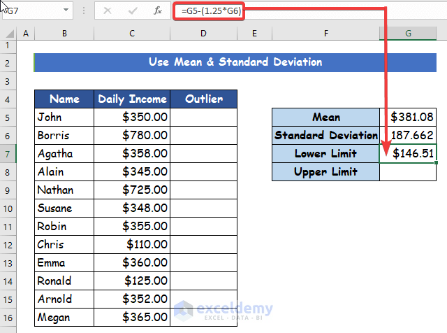
Step 4:
- In cell G8, calculate the upper limit from the following formula:
=G5+(1.5*G6)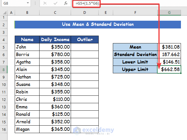
Step 5:
- Enter the following formula in cell D5 to calculate whether any outliers exist:
=OR(C5<$G$7,C5>$G$8)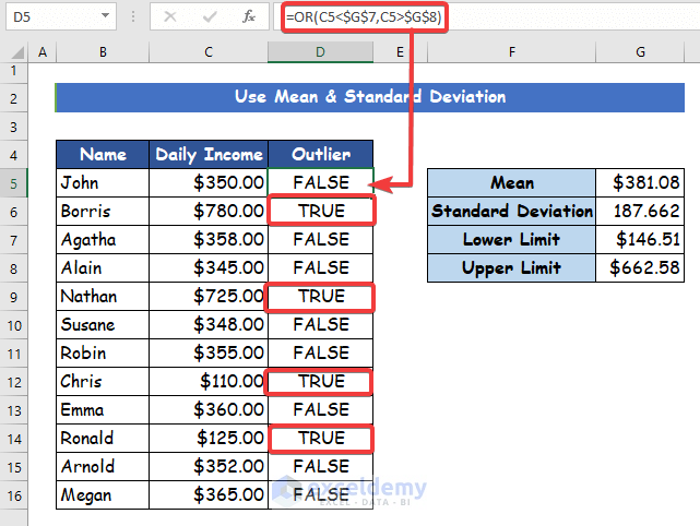
- The formula will return a TRUE value if the specific data in the desired cell is an outlier and FALSE.
- Double-click on the AutoFill tool in cell D5 to copy the formula to the rest of the cells in column D. You can find all the remaining outliers in your dataset.
Read More: How to Find Outliers with Standard Deviation in Excel
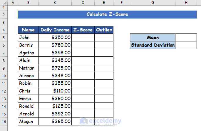
Method 4 – Inserting Z-Score to Calculate Outliers in Excel
Step 1:
- Use the desired dataset.
Step 2:
- In cell H5, enter the following formula to calculate the mean for the given data:
=AVERAGE(C5:C16)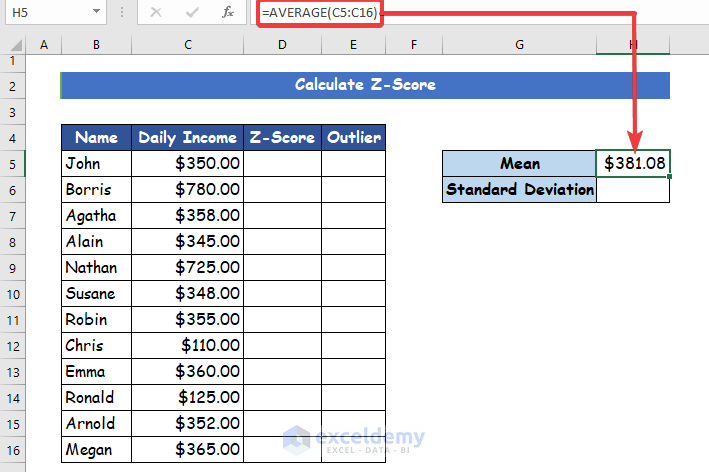
Step 3:
- Calculate the standard deviation of the given dataset in cell H6 by using the following formula:
=STDEV.P(C5:C16)
Step 4:
- Determine the Z-score for each data value. To do this, use the formula given below:
=(C5-$H$5)/$H$6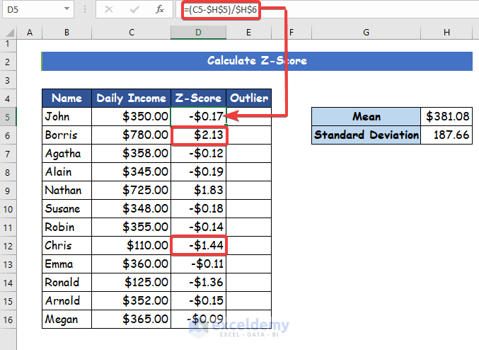
Step 5:
- After calculating all the Z-values, you will see that the range of Z-values is between -1.44 and 13. So, we consider values of Z-score less than -1.2 or more than +1.8 for the outlier limits.
- Enter the following formula into cell E5:
=OR((D5<-1.2),(D5>1.8))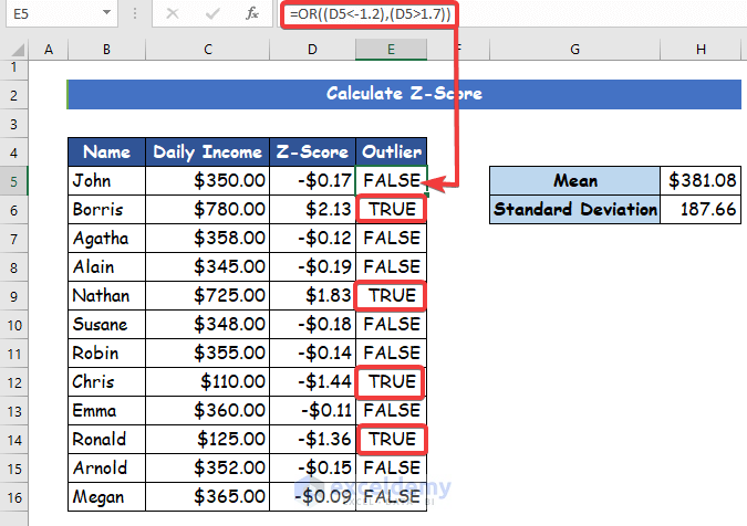
- Finally, the formula will return a TRUE value if the specific data is an outlier and will return a FALSE
- Double-click on cell E5 to use the AutoFill tool fill handle to copy the formula to the rest of the cells in column E. Thus, you can find all the remaining outliers in your dataset.
Read More: How to Find Outliers Using Z Score in Excel
Method 5 – Merging LARGE and SMALL Functions to Find Outliers in Excel
Step 1:
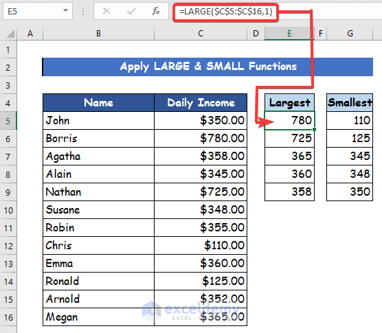
- Enter the following formula in cell E5 with the LARGE function:
=LARGE($C$5:$C$16,1)-
- From 12 values, you can see the 1st largest value, which is 780.
Step 2:
- In cell G5, enter the following formula to find the smallest value:
=SMALL($C$5:$C$16,1)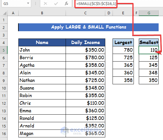
- From 12 values, you can see the 1st smallest value, 110.
- Once you have found all the required values, you can easily point out any outliers in the dataset.
Download the Practice Workbook
You can download the free Excel workbook from here and practice.

