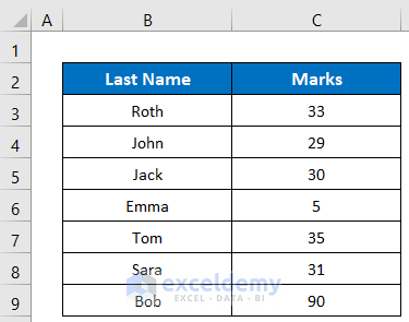
This is the sample dataset.
Method 1 – Removing Outliers Manually in an Excel Scatter Plot
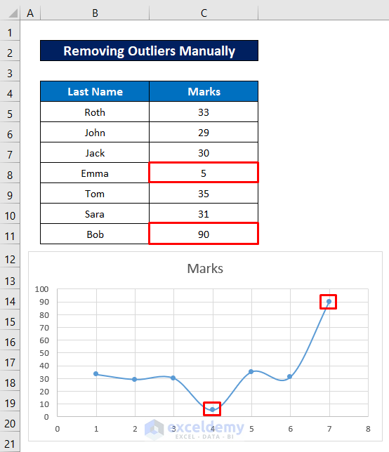
Steps:
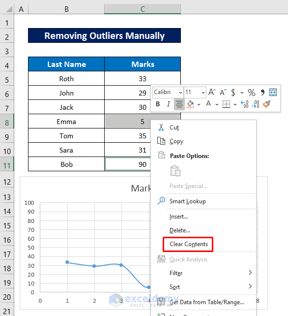
- Press and hold CTRL key and click the values one by one.
- Right-click and select Clear Contents or press DELETE.
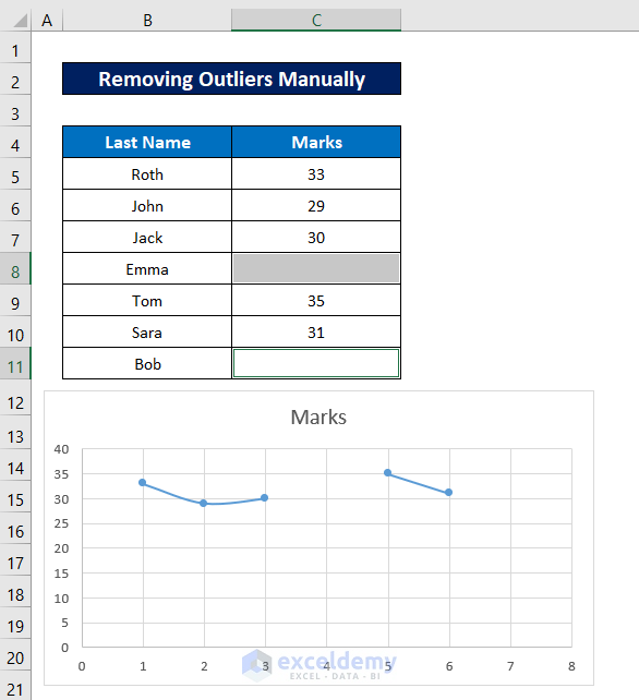
As the values were deleted, the graph became discontinued.
Read More: How to Show Outliers in Excel Graph
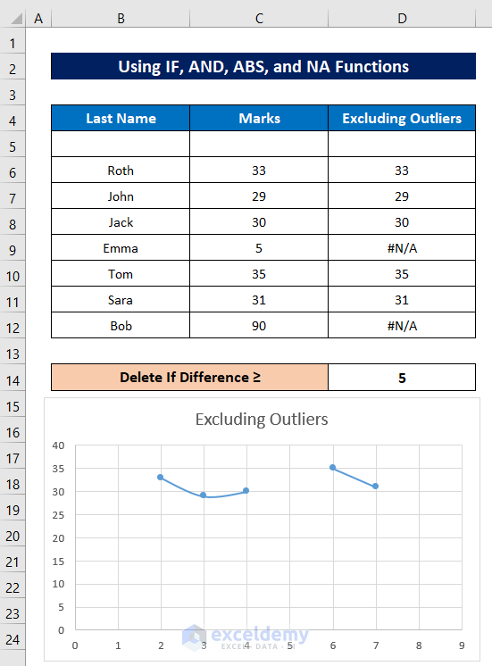
Method 2 – Using the Excel IF, AND, ABS, and NA Functions to delete Outliers in Scatter Plot
Column D was added.
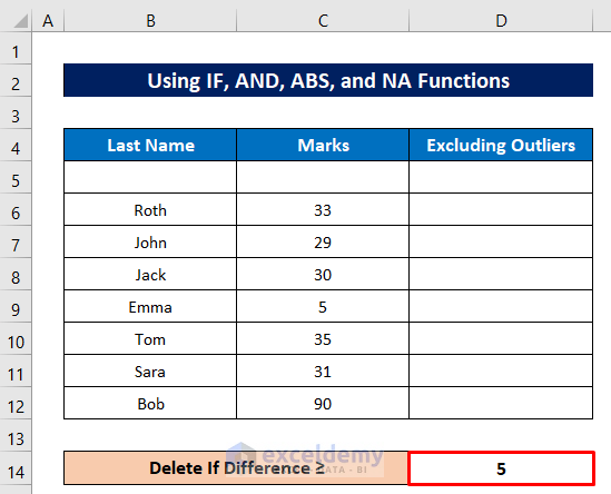
Steps:
- Enter the following formula in D6.
=IF(AND(ABS(C6-C5)>$D$14,ABS(C6-C7)>$D$14),NA(),C6)- Press Enter to see the output.
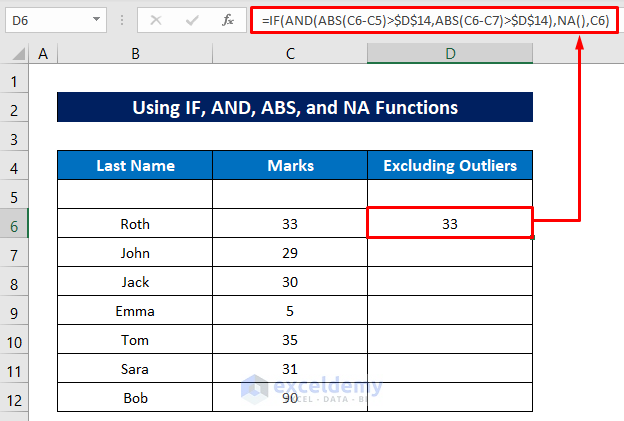
Formula Breakdown:
- ABS(C6-C7)>$D$14
The ABS function finds the absolute difference between C6 and C7. It checks whether the output is greater than the specified difference, which will return:
FALSE
- ABS(C6-C5)>$D$14
It finds the absolute difference between C6 and C5. It checks whether the output is greater than the specified difference, which will return:
TRUE
- AND(ABS(C6-C5)>$D$14,ABS(C6-C7)>$D$14)
The AND function combines the outputs and returns:
FALSE
- IF(AND(ABS(C6-C5)>$D$14,ABS(C6-C7)>$D$14),NA(),C6)
The IF function performs the logical test. If the previous outputs return TRUE, it will display the #N/A error. If FALSE, it will show the exact value of C6. For D6, it will return:
33
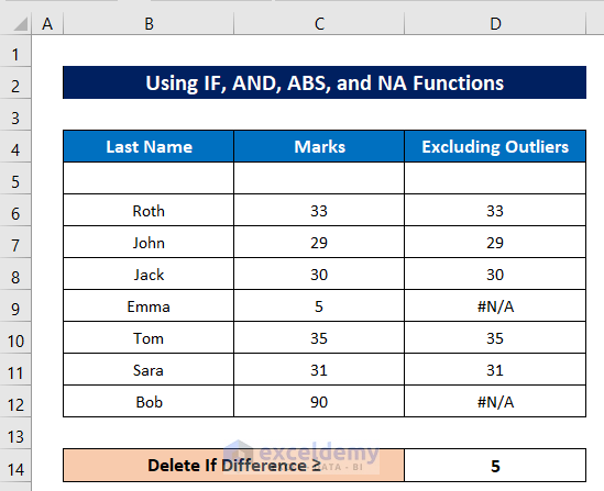
- Drag down the Fill Handle to see the result in the rest of the cells.
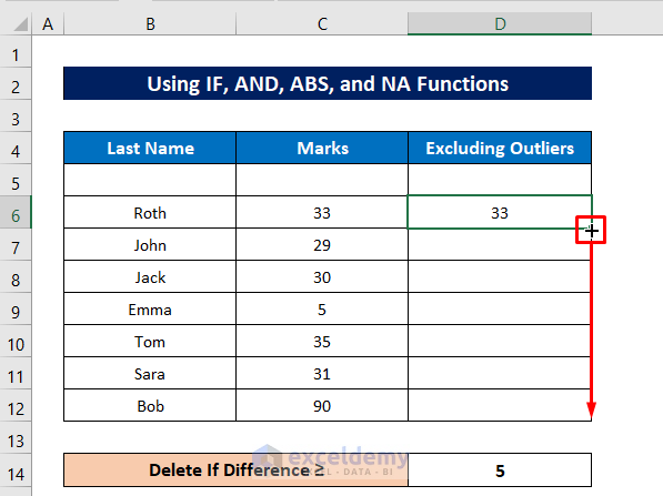
The most deviated values are removed.
- Select the new column and create a Scatter Plot chart
Outliers are removed from the Scatter Plot chart.
Read More: How to Calculate Outliers in Excel
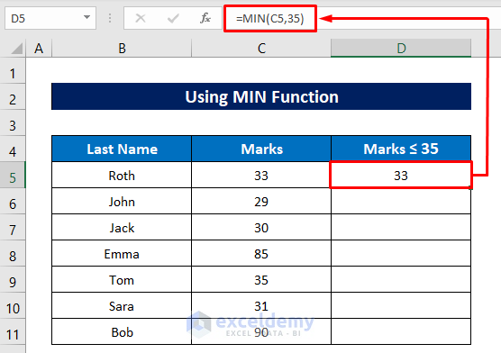
Method 3 – Using the MIN Function to Delete Outliers in a Scatter Plot
Steps:
- In D5, enter the following formula:
=MIN(C5,35)- Press Enter to see the result.
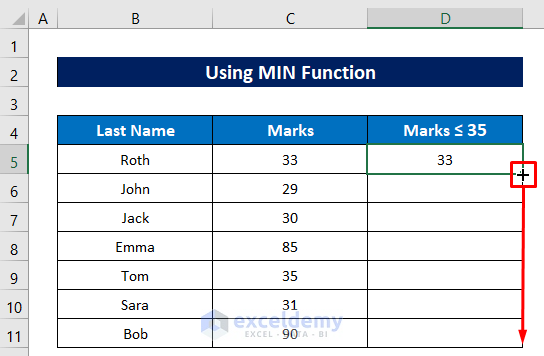
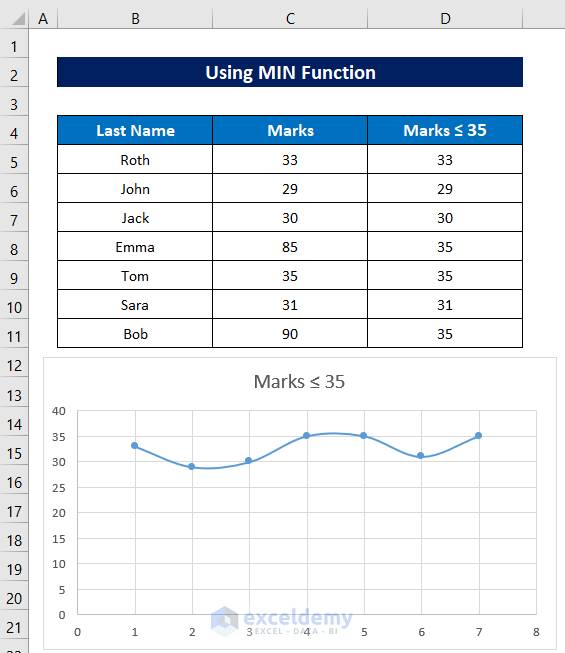
- Drag down the Fill Handle to see the result in the rest of the cells.
- Insert a Scatter Plot chart for the new column and you will get a smooth and continuous chart:
Download Practice Workbook
Download the free Excel workbook.
Related Articles
- How to Find Outliers Using Z Score in Excel
- How to Find Outliers in Regression Analysis in Excel
- How to Find Outliers with Standard Deviation in Excel
<< Go Back to Outliers in Excel | Excel for Statistics | Learn Excel
Get FREE Advanced Excel Exercises with Solutions!
