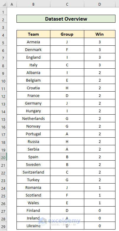
This is the sample dataset.
Method 1 – Combining the Excel INDEX-SMALL Formula to Filter Data
The INDEX function returns the value at a given location in a range or array.
INDEX (array, row_num, [col_num], [area_num])array: A range of cells, or an array constant.
row_num: The row position in the reference or array.
col_num: The column position in the reference or array. This is an optional field.
area_num: The range that should be used in the reference. This is an optional field.
The SMALL function returns numeric values based on their position in a list ranked by value.
SMALL (array, n)array: A range of cells from which to extract the smallest values.
n: An integer that specifies the position of the smallest value: the nth position.
Combining the IFERROR and the ROW functions.
The generic formula is:
IFERROR(INDEX(return_array,SMALL(IF(criteria_check, ROW(criteria_array),""),ROW()-ROW(starting_row))),"")IFERROR encloses the nested formula to avoid errors.
row_number is is included in the INDEX function using the SMALL function.
In the SMALL function, the array is set within the IF function.
- Enter the formula:
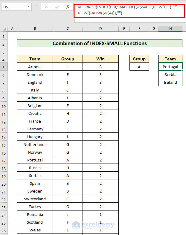
The return_array is the Team column. The formula checks whether Group A matches the Group column. This logical test returns an array of TRUE or FALSE. TRUE if criteria are met, FALSE otherwise. ROW(C: C) returns the row numbers of column C in an array if_true_value of the IF function. Otherwise, empty strings.
(IF(criteria_check, ROW(criteria_array),"") returns an array of “” and row number.
ROW()-ROW(starting_row) returns the incremental number of rows: the n in the SMALL function, which returns a row index value used by the INDEX function to return a value from a non-empty cell.
- Press CTRL + SHIFT + ENTER.
This is the output.
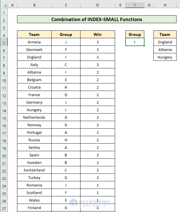
Group I is selected.
The generic formula is:
IFERROR(INDEX(return_array,SMALL(IF(criteria_check, ROW(return_array)-ROW(starting_row)+1,""),ROWS(starting_row:present_row))),"") Two ROW functions are used to return the row number from the starting row. The ROWS function returns the incremental number of rows.
- Enter the formula.
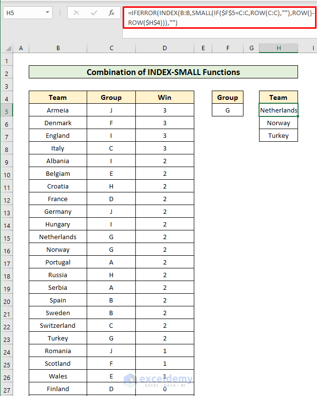
- Press CTRL + SHIFT + ENTER.
This is the output.
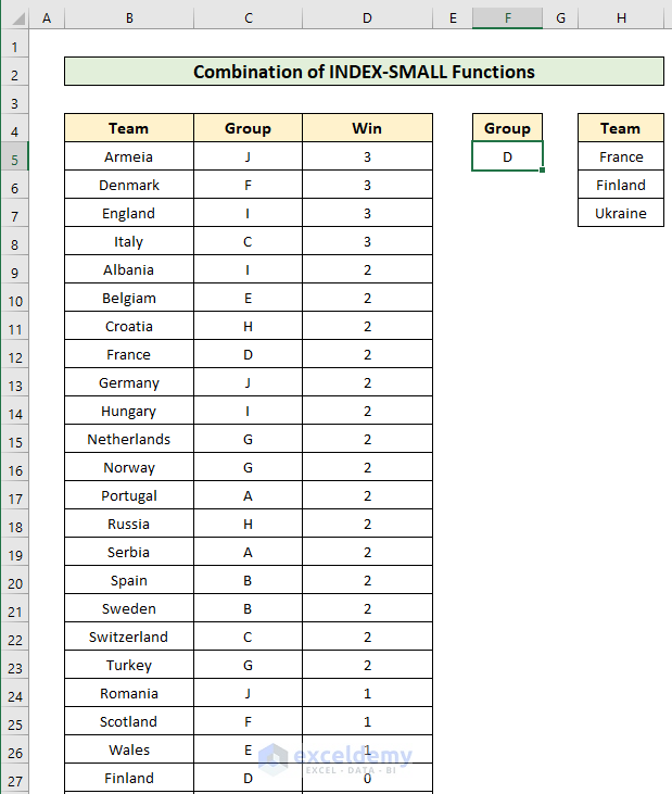
To change the criteria from Group to Win, change the criteria_array.
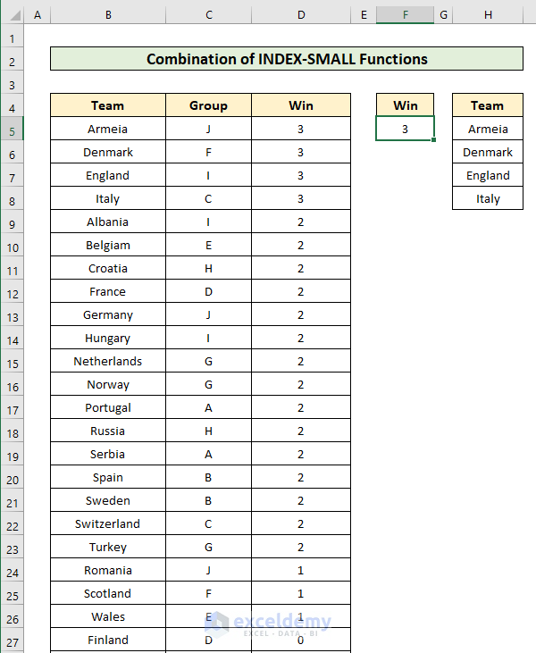
This is the output.
Method 2 – Using the Excel FILTER Function to Filter Data
The FILTER function filters a range of data based on criteria and extracts matching records.
FILTER (array, include, [if_empty])array: Range or array to filter.
include: Boolean array, supplied as criteria.
if_empty: Value to return when no results are returned. This is an optional field.
Filtering with a Single Criterion
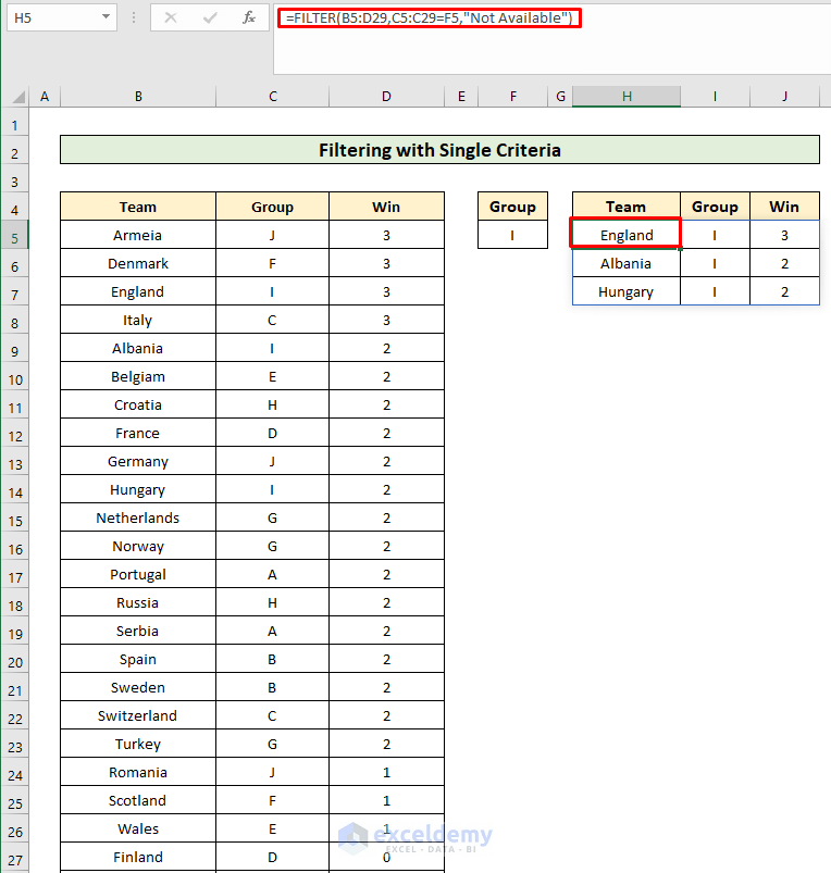
The entire table is the array. The formula checks whether the Group column has the criteria Group I and returns three teams. “Not Available” was used in the if_empty field.
Filtering with Multiple Criteria
FILTER(array, (range1=criteria1) * (range2=criteria2), if_empty)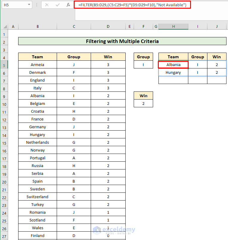
The two criteria are Group and Win. The formula checks the criteria values and multiplies them. It returns the teams from group I with 2 wins. The plus sign symbol (+) is used to denote the OR logic.
FILTER(array, (range1=criteria1) + (range2=criteria2), if_empty)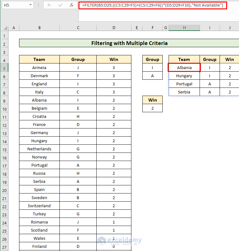
The formula checks the criteria values and adds them before multiplying them by the Win criteria. It returns the teams in group I and all teams with 2 wins. The AND-OR logic is used.
Filtering Dates
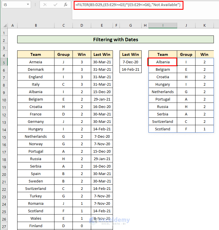
The Last Win column was inserted. The conditions (equal or greater than the starting date and less or equal to the end date) were set and multiplied to return the teams whose Last Win is between 7 December 2020 and 14 February 2021.
Filtering Duplicates
- Use the formula:
FILTER(array, COUNTIFS(column1, column1, column2, column2,...)>1, if_empty)
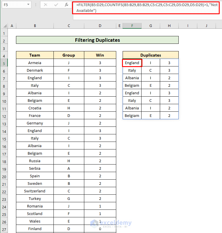
The columns are inserted in the COUNTIFS function.
Filtering Blanks
- Enter the formula:
FILTER(array, (column1<>"") * (column2=<>"")*..., if_empty)
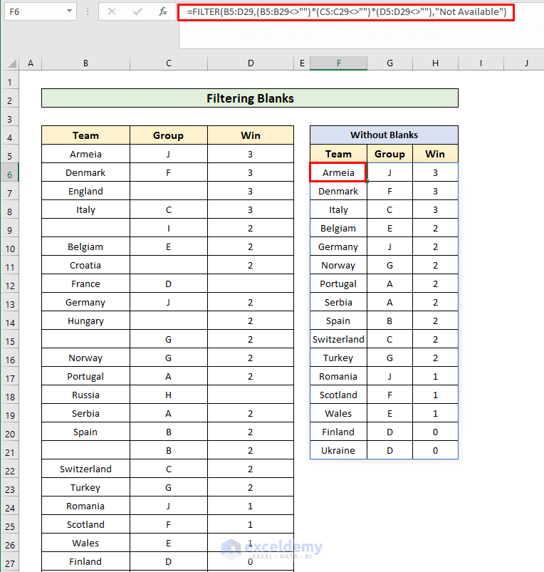
There are empty cells in the dataset. The formula identifies non-blank cells, using the “not equal to” operator (<>) with an empty string (“”) and returns the result without blank or empty cells.
Filtering Non-adjacent columns
- Enter the formula:
FILTER(FILTER(array,include),{1,0,1})
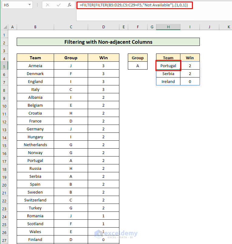
{1,0,1} is the include field for the outer FILTER. 1 refers to the columns to be kept and 0 to the columns to be excluded.
Instead of 1 and 0, you can use TRUE or FALSE.
Filtering a Number of Rows
[wpsm- Use the formula:
_box type=”solid_border” float=”none” textalign=”left” width=”60%” ]
INDEX(FILTER(array,include),{1;2},{1,2,3})
[/wpsm_box]
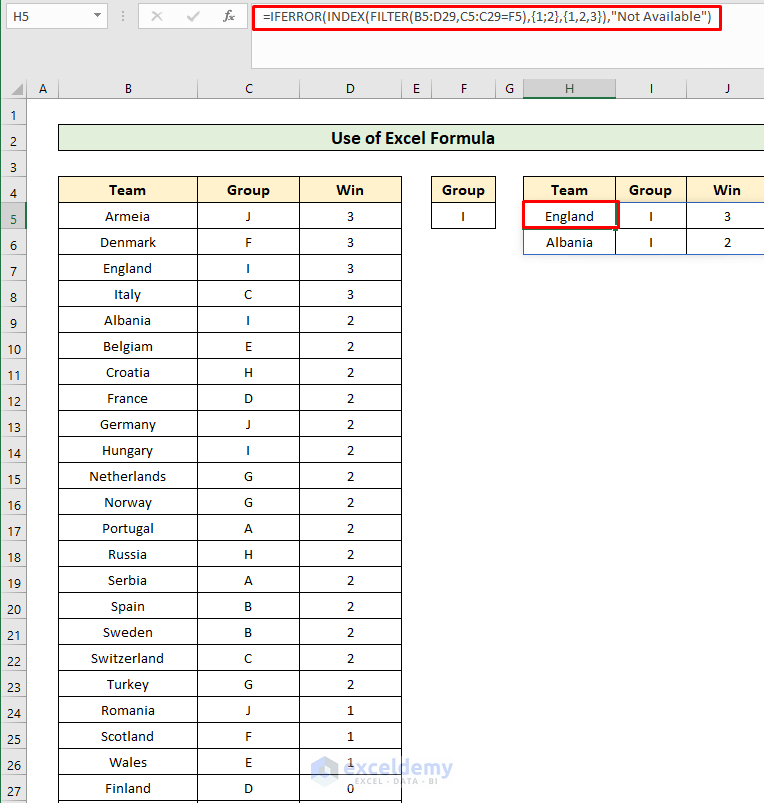
Use {1;2} or {1,2,3} and insert your values.These are the row_number and the column_number of the INDEX function. It returns the rows and columns. The formula is wrapped the with IFERROR to avoid errors.
Practice Workbook
Download the practice workbook.

