This is an overview.

Create Data Connections between Excel Files
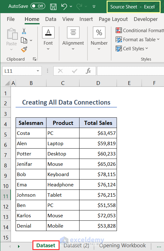
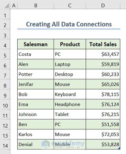
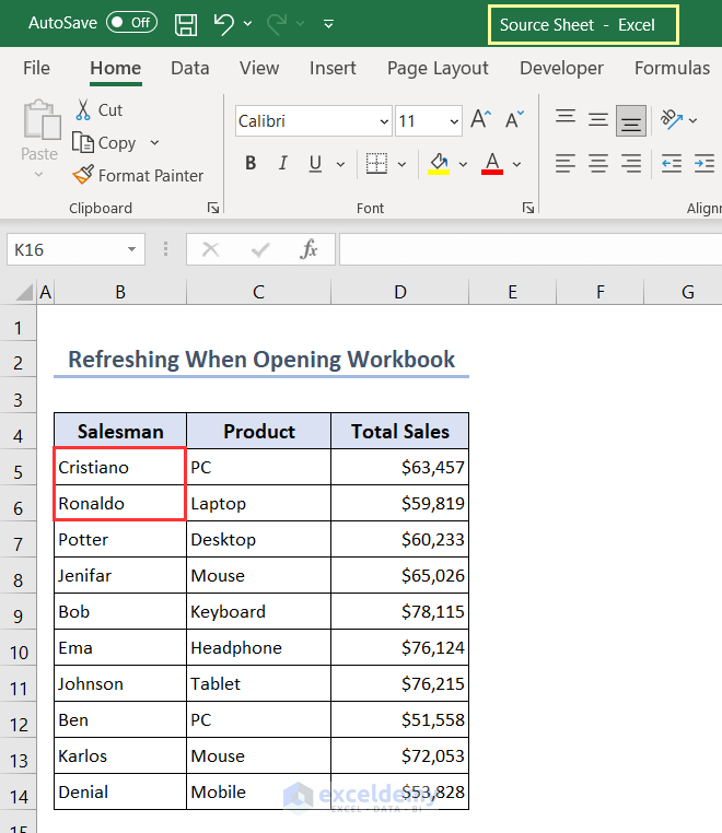
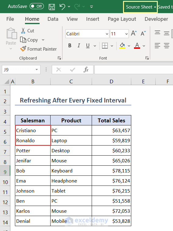
The original dataset is the Dataset sheet in the Source Sheet workbook .
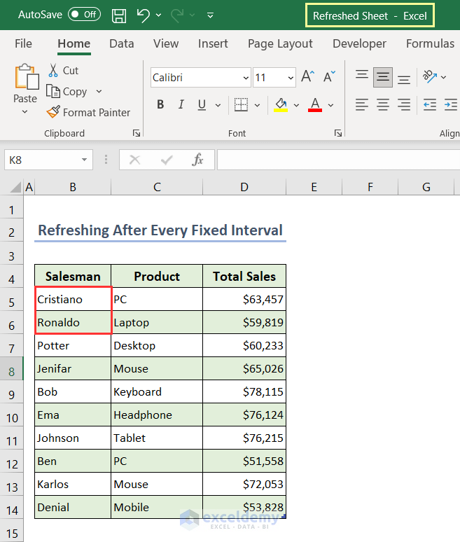
- Upload this dataset to a new book: Refreshed Sheet.
- In the Refreshed Sheet, go to Data > Get Data > From File > From Excel Workbook.
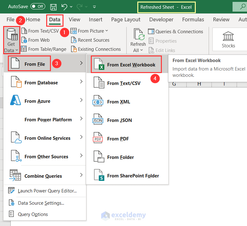
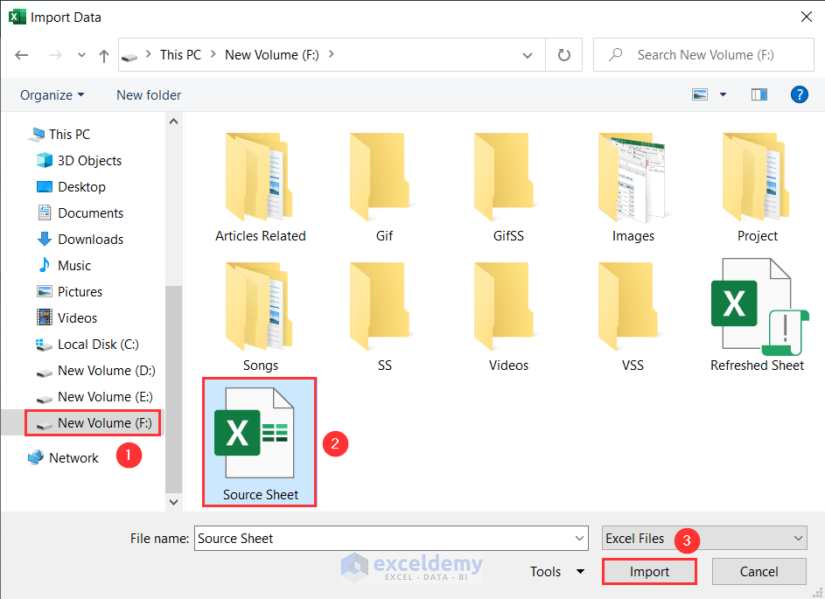
- Choose the file you want to upload.
- Here, Source Sheet from New Volume (F:).
- Click Import.
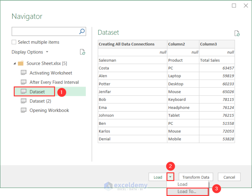
- In the Navigator window select the sheet containing the dataset you want to upload. Dataset, here.
- Go to Load and click Load To.
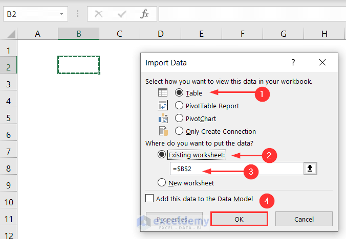
- In the Import Data window select Table.
- Choose Existing worksheet: to provide the position of the dataset and enter B2.
- Click OK.
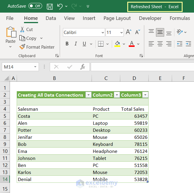
- Your data will be uploaded to the Refreshed Sheet in table format. It’ll be connected with the Source Sheet.
- You can format the dataset:
How to Refresh All Data Connections Using Excel VBA – 4 Examples
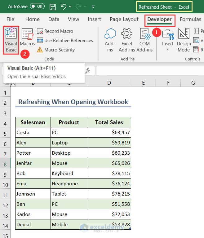
Example 1 – Refreshing When Opening Workbook
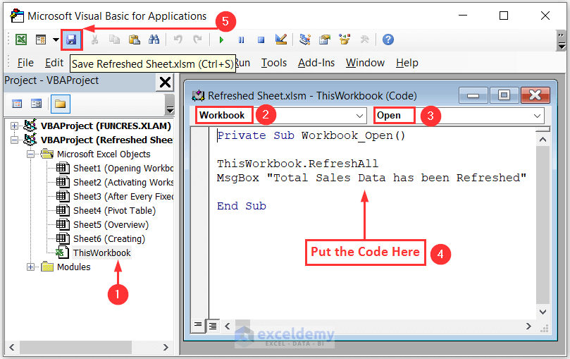
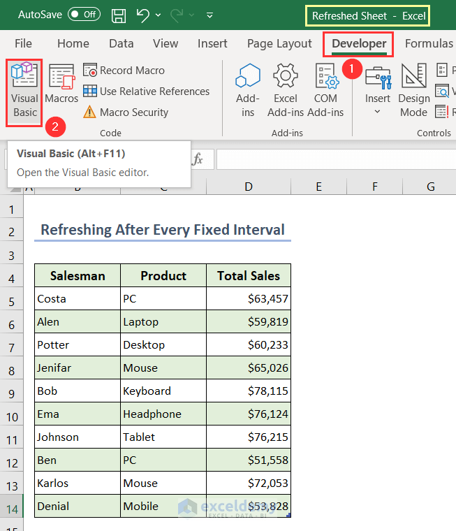
- Open the workbook Refreshed Sheet and go to Developer > Visual Basic. You can also use Alt + F11 to open Visual Basic.
- Double-click ThisWorkbook.
- Choose Workbook > Open > Module and enter the following code.
Private Sub Workbook_Open()
ThisWorkbook.RefreshAll
MsgBox "Total Sales Data has been Refreshed"
End Sub- Click Save or press Ctrl + S. You don’t have to run the code.
- Close the Refreshed Sheet.
- Open the Source Sheet and change the two first names in Salesman.
- Save and close.
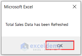
- Open the Refreshed Sheet. This message will be displayed.
- Click OK.
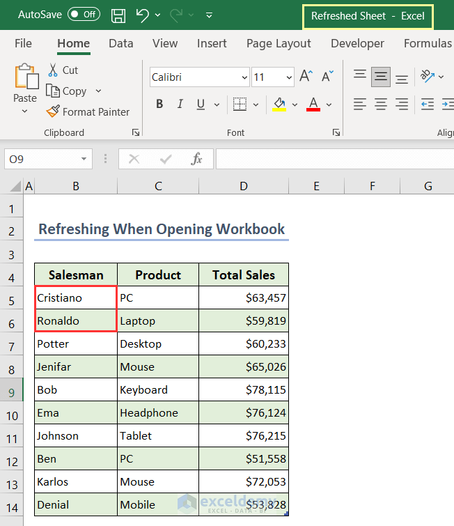
The dataset is automatically refreshed .
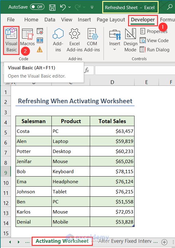
Example 2 – Refreshing When Activating the Worksheet
- Select Visual Basic in the Developer tab in the Activating Worksheet (Refreshed Sheet workbook). You can also use Alt + F11 to open the Visual Basic.
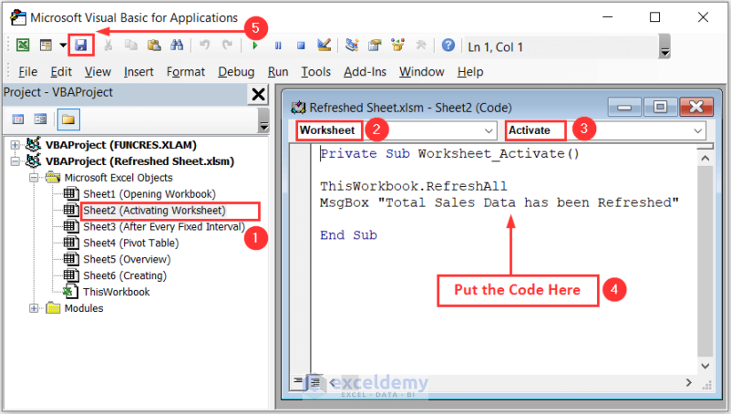
- Double-click Sheet2 (Activating Worksheet).
- Choose Module> Worksheet >Activate and enter the following code.
Private Sub Worksheet_Activate()
ThisWorkbook.RefreshAll
MsgBox "Total Sales Data has been Refreshed"
End Sub- Click Save or press Ctrl + S. You don’t have to run the code.
- Close the Refreshed Sheet.
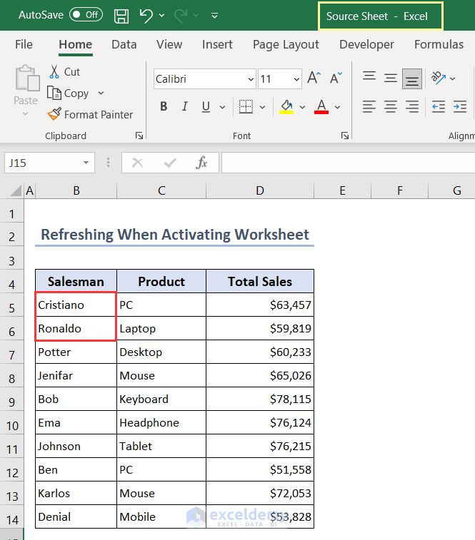
- Change the two first names in Salesman in the Source Sheet.
- Save and close.
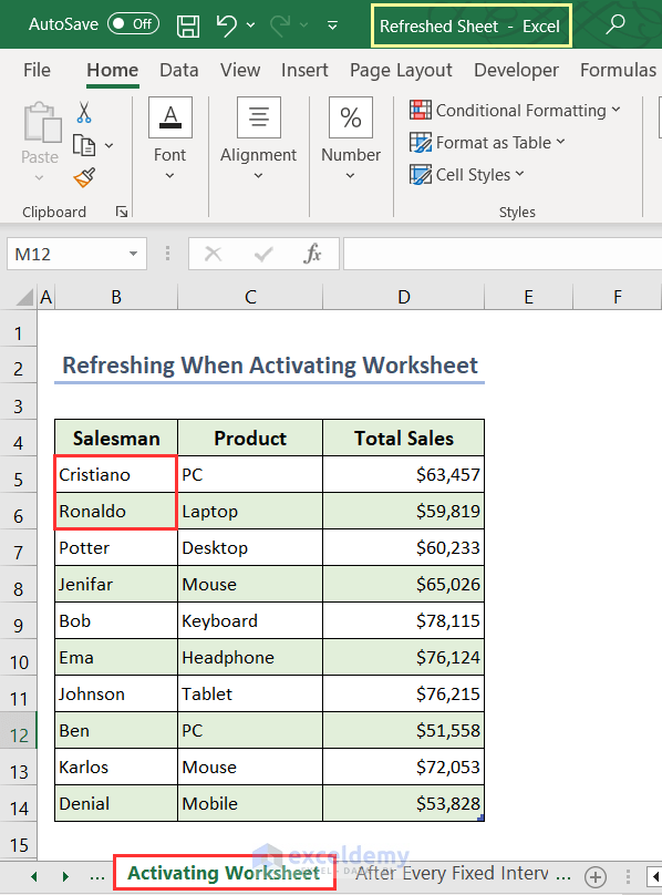
- Open the Refreshed Sheet and activate the Activating Worksheet. This message will be displayed.
- Click OK.

The dataset is automatically updated.
Example 3 – Refreshing After a Fixed Interval with VBA
60 seconds or 1 minute is the fixed interval, here.
- In the Refreshed Sheet select Visual Basic in the Developer tab.
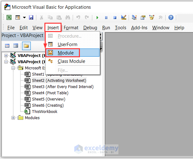
- In Visual Basic choose Insert and select Module.
- Enter the following code and click Run or press F5 to run the code.
Public ReloadInterval As Double
Public Const Period = 60
Sub Reload()
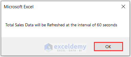
MsgBox "Total Sales Data will be Refreshed at " & _
"the interval of " & Period & " seconds"
Call FirstReload
End Sub
Sub FirstReload()
ReloadInterval = Now + TimeSerial(0, 0, Period)
Application.OnTime _
EarliestTime:=ReloadInterval, _
Procedure:="ReloadConnections", _
Schedule:=True
End Sub
Sub ReloadConnections()
ThisWorkbook.RefreshAll
Call FirstReload
End Sub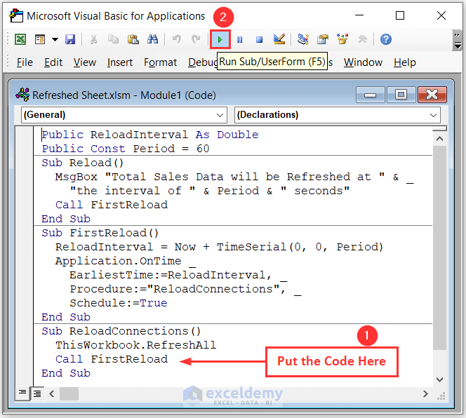
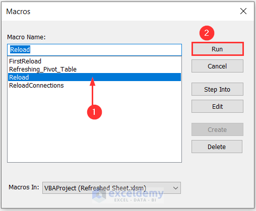
- The Macros window will open.
- Select Reload and click Run.
- This message will be displayed. Click OK.
- In the Source Sheet, change the two first names in Salesman. Save and close.
- Wait 60 seconds and open the Refreshed Sheet.
Data is automatically refreshed after every 60 seconds or 1 minute.
Read More: How to Refresh Data Connection in Excel Without Opening File
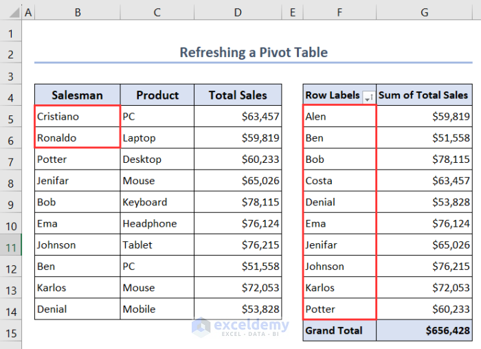
Example 4 – Refreshing a Pivot Table
- This is the Pivot Table.
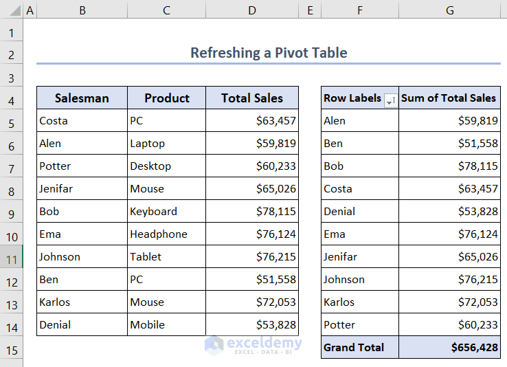
- Changing the two first names in Salesman won’t change data in the Pivot Table. It must be refreshed.
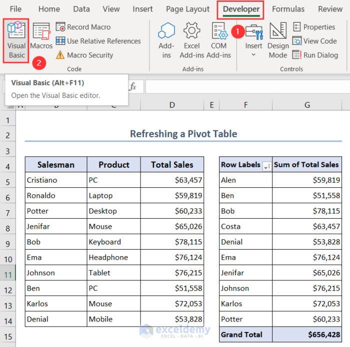
- Select Visual Basic in the Developer tab.
- In Visual Basic choose Insert and select Module.

- Enter the following code and click Run or press F5 to run the code.
Sub Refreshing_Pivot_Table()
ActiveSheet.PivotTables("PivotTable1").RefreshTable
End Sub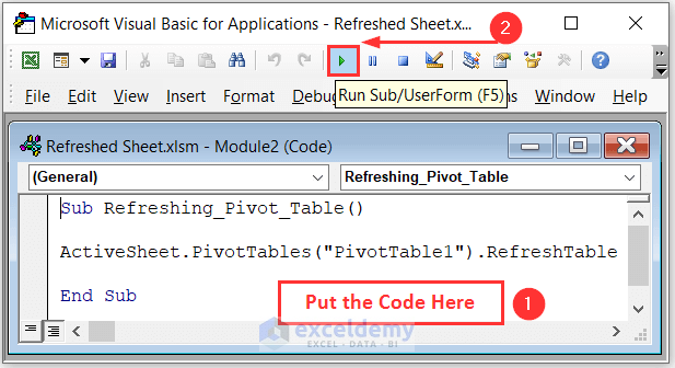
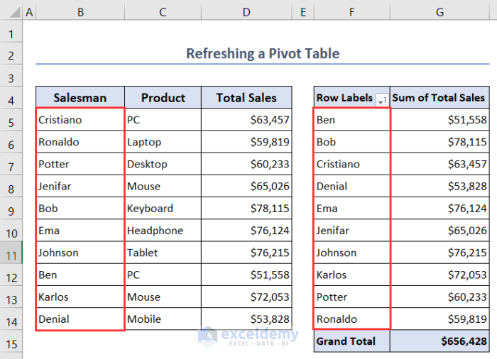
The Pivot Table is refreshed.
Read More: [Fixed]! Data Connection Not Refreshing in Excel
Download Practice Workbook
Download the Excel files and practice.
Related Arrticles
- How to Create a Data Source in Excel
- [Fixed!] External Data Connections Have Been Disabled in Excel
- Excel Connections vs Queries
- [Solved!] Excel Queries and Connections Not Working
<< Go Back to Excel Data Connections | Importing Data in Excel | Learn Excel
Get FREE Advanced Excel Exercises with Solutions!

Greetings,
We’re experiencing an issue with a supplier who has failed to comply with our sales agreement. We’d like to explore options for resolving this matter.
Could you please advise if you’re equipped to handle this situation? We’re seeking professional guidance to navigate this dispute and find a suitable solution.
Thank you for your prompt attention to this matter.
Best regards,
AM
Hello Alex Minta,
Thank you for your message. Our site is focused on learning resources, tutorials, and guidance to help users build their own skills. We don’t directly handle legal disputes with suppliers, but we can share knowledge on how to structure agreements, manage compliance, and use tools (like Excel) to monitor and document business activities.
If you need formal dispute resolution, it’s best to consult a legal or compliance professional. However, you’ll find our guides helpful for learning how to better manage supplier records and agreements in the future.
Regards
ExcelDemy