How to Make Union of Two Sheets in Excel (4 Suitable Methods)

Get FREE Advanced Excel Exercises with Solutions!

For work purposes, data entries in Excel by different employees in various worksheets may be a root cause of discomfort for some officials who prefer to see the different entries in a single Excel worksheet. So, to solve the problem we have got various solutions. The best approach in this regard is to use the Excel union. In this article, I will show you 4 effective methods to perform union between two sheets in Excel.

Table of Contents hide

Download Practice Workbook

4 Effective Methods to Make Union of Two Sheets in Excel

1. Unify Two Sheets Using Consolidate Feature

2. Using VLOOKUP Function to Make a Union

3. Use Power Query to Perform a Union Between Two Sheets

4. Applying VBA to Make a Union of Two Sheets in Excel

Conclusion

Download Practice Workbook

You can download the practice workbook from the following download button.

Union Two Sheets.xlsm

4 Effective Methods to Make Union of Two Sheets in Excel

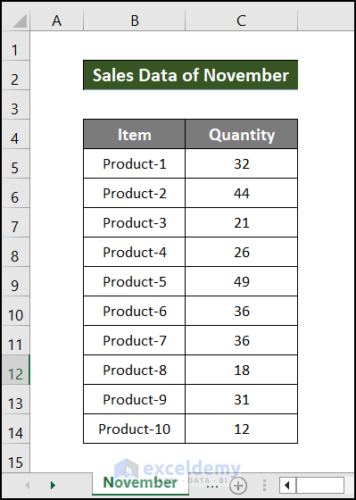
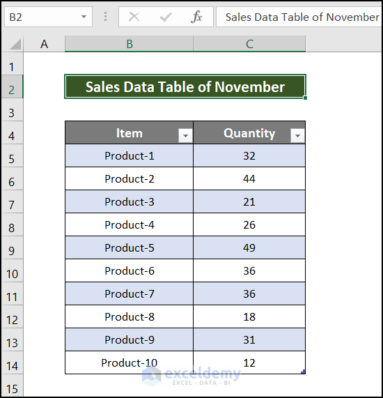
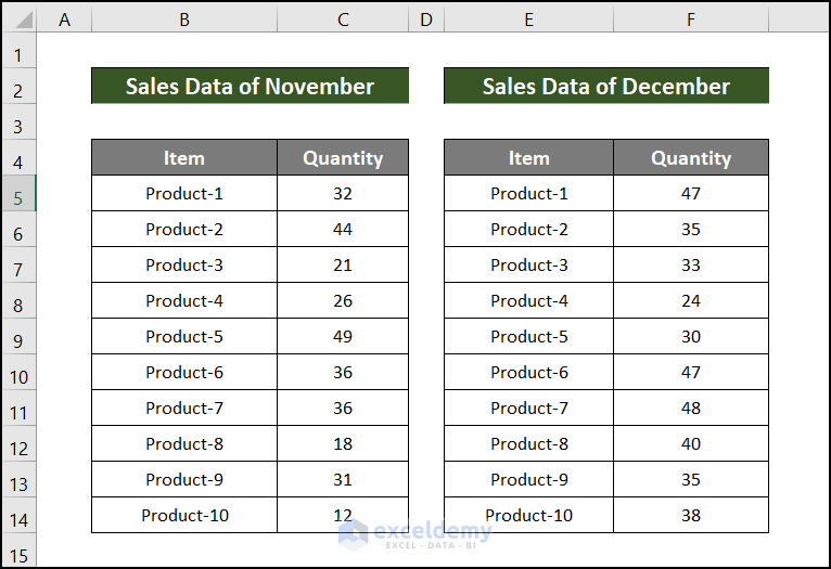
The Quantity of 10 products for November and December is the dataset we use in the first scenario. The name of the Products and quantities for November are located in cells B5 through C14 of the November sheet.

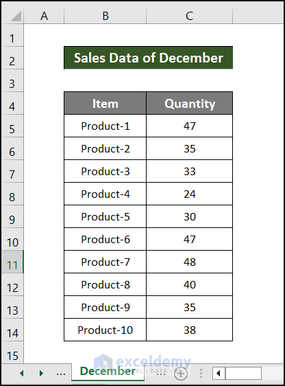
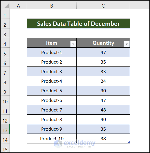
Again, the name of Products and their Quantity for December are located in cells B5 through C14 of the December sheet.

1. Unify Two Sheets Using Consolidate Feature

To get the solution from Excel Tab we have Consolidate option to merge data in Excel. In this method, we are going to demonstrate the merging of data into one sheet from two different sheets.

📌 Steps:

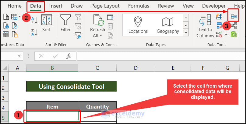
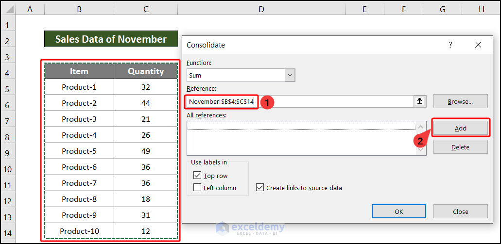
Select cell B5 from where consolidated data will be displayed.
Then follow the steps: Data >> Consolidate.

As a consequence, Consolidate, a little dialog box, will show up.
Keep the Function in Sum after that.

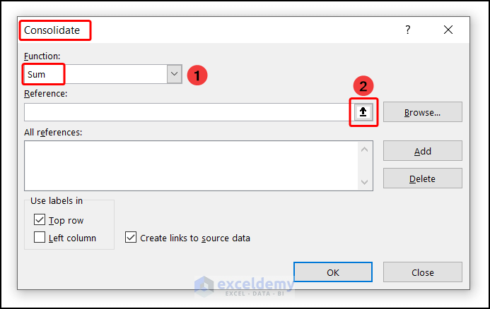
After that, choose the November sheet’s cells B4:C14 from the Reference box.
Then choose Add.

Similarly, select the December sheet’s cells B4:C14 from the Reference box.
Now, click Ok.

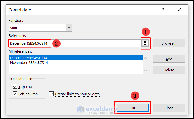
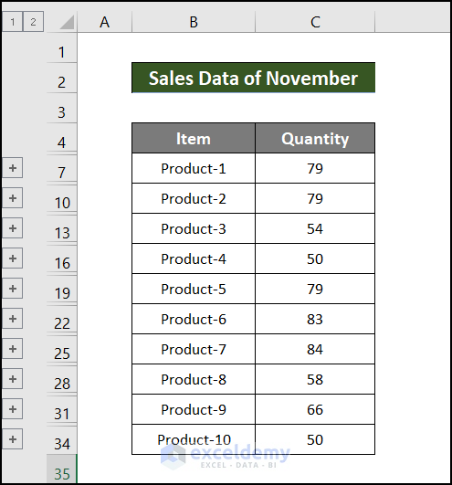
Finally, we will be able to perform a union between two sheets and will get the combined data from two sheets to one.

Note:

In this method, you have to ensure the same size of the table in both worksheets. And those tables must be located in the same cells in the two source worksheets.

2. Using VLOOKUP Function to Make a Union

In this case, we’ve used the VLOOKUP function to merge the data from the two sheets into a single sheet.

📌 Steps:

As we have to combine two datasets, we can do that using the VLOOKUP function.
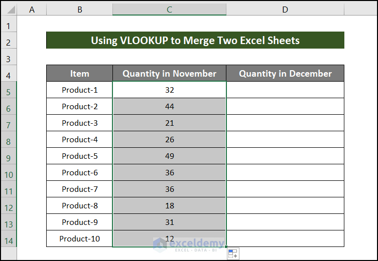
To do so we will enter the following equation in cell C5.

=VLOOKUP(B5,November!B5:C14,2,FALSE)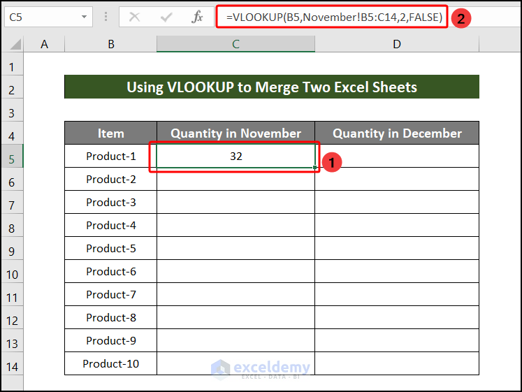

Press Enter and move the Fill Handle Tool downward.

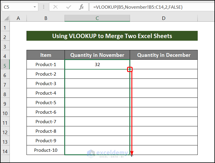
Our desired Quantity in November column will look like the following image.

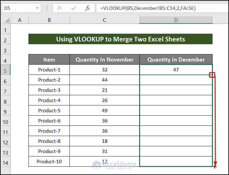
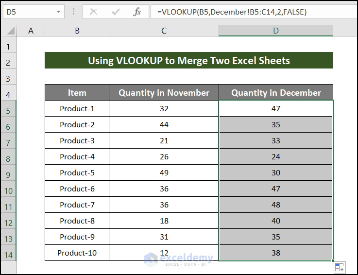
The VLOOKUP function can be used to join two datasets, which is what we are going to do.
To achieve this, we will type the equation below into cell D5.

=VLOOKUP(B5,December!B5:C14,2,FALSE)

After entering the equation, we will drag the fill handle down to copy the formula for the rest of the cells.

Thus, we have made a union of two Excel sheets.

Note:

In doing this, there must be a common column in both sheets. The VLOOKUP will work on that column as a lookup value and return values from individual sheets.

3. Use Power Query to Perform a Union Between Two Sheets

In Excel, we have Power Query to merge data in Excel. In this method, we are going to demonstrate the merging of data into one sheet from two different sheets by Power Query.

📌 Steps:

Before getting into Power Query, we have to turn our dataset into a Table by following the path: Insert >> Table.

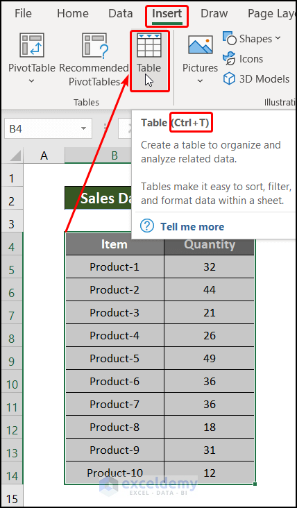
Then our dataset converted to a table and will look like the below image.

Similarly, to the previous stage, we will turn the December dataset into a Table and the result will look like the below image.

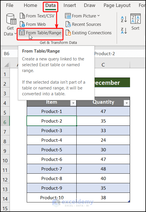
Select a cell from the table of November.
Now go to the Data tab and click on the From Table/Range.

After selecting the From Table/Range, a Table1- Power Query Editor will open up.
Here, we will not edit anything just follow the path: Home >> Close & Load >> Close & Load To…

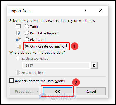
Immediately after selecting Close & Load To…, a window will be opened to determine how the Close & Load operation will be done.
The name of the window is Import Data.
From the window Import Data, we will choose Only Create Connection and then select Ok.

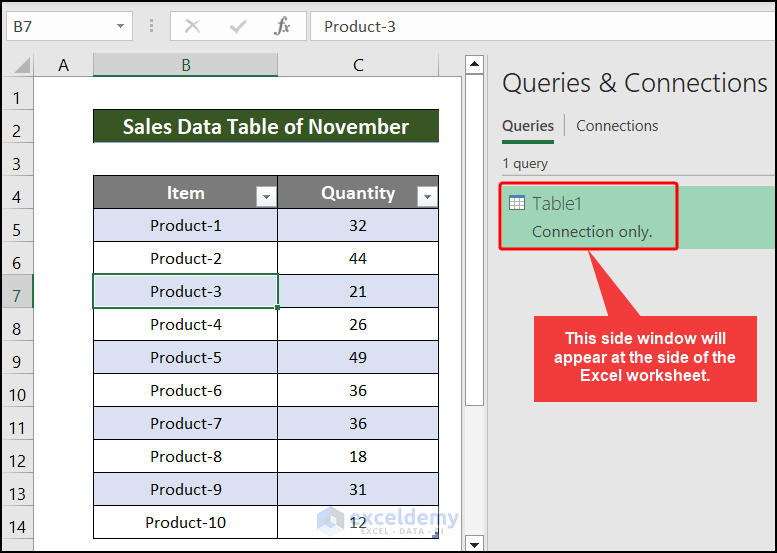
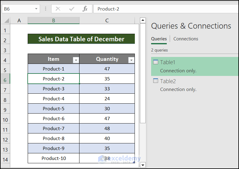
Now after choosing Close & Load To…, the Queries & Connection side window will be opened in the sidebar of our current worksheet.
Under Queries, we will see Table1(Connection Only).

Choose a cell from the December table.
And for now, go to the Data tab and choose “From Table/Range.”

A Table2- Power Query Editor will pop up after choosing From Table/Range.
Like in the previous steps, we won’t modify anything now; simply go as follows: Home >> Close & Load >> Close & Load To…

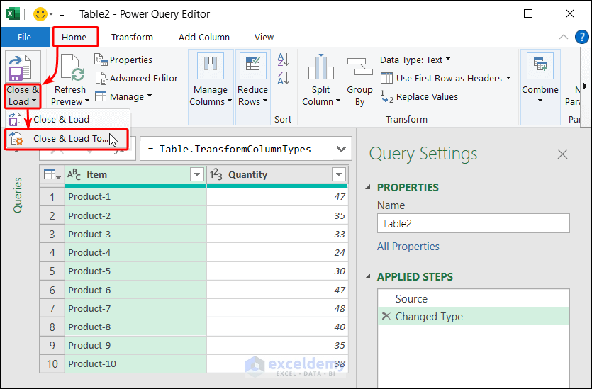
As soon as we choose Close & Load To…, a window will appear to provide the Close & Load operation’s parameters.
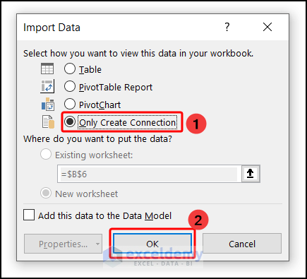
Import Data is the title of the window.
We will pick the Only Create Connection option from the Import Data box, then click OK.

The Queries & Connection side window will now be presented on the sidebar of our current worksheet after selecting Close & Load To…
Table2 will be found under Queries (Connection Only).

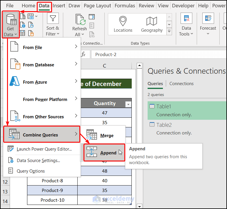
After the Close & Load operation is done, we will combine those data tables in a vertical combination.
To do so, we will follow the path: Data >> Get Data >> Combine Queries >> Append.

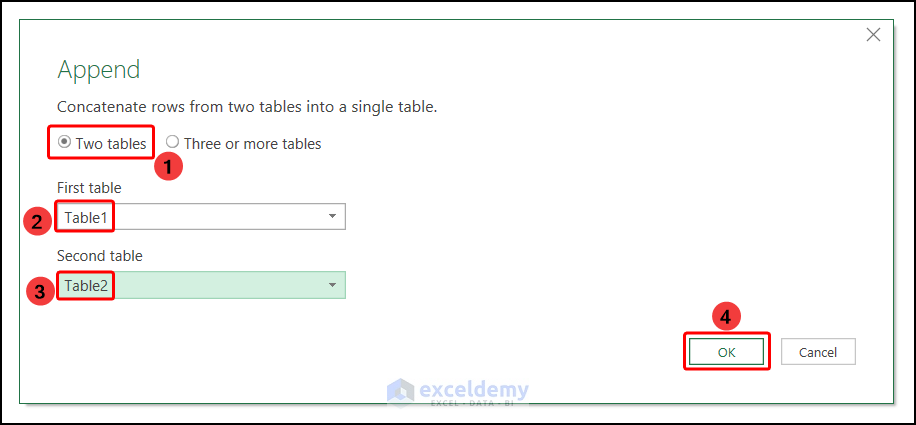
Now just after Close & Load, the Append window will appear.
As we are demonstrating excel union two sheets with two tables, we are going to select Two tables under the line of Concatenate rows from two tables into a single table just like the steps shown in the below image.
Now for the First Table select Table1 and for the Second Table choose Table2.

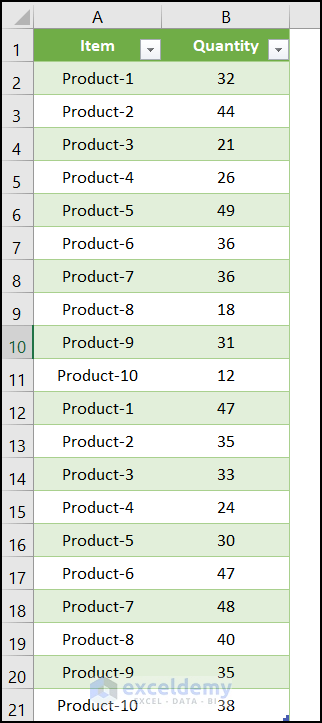
Now in the Power Query, the consolidated data will look like the below image.
To insert the data in the Excel worksheet, we are going to select Close & Load.

Finally, we have a table from two different sheets that are stacked one after another.

4. Applying VBA to Make a Union of Two Sheets in Excel

Now we’ll create a macro to laterally integrate the two worksheets into a single worksheet.

Open the worksheet where you wish to combine these files. I’ve opened a worksheet here named Union Sheets Using VBA. Then, follow the steps below to accomplish this.

📌 Steps:

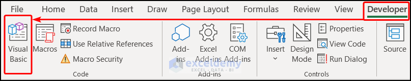
Firstly, go to the Developer tab and choose the Visual Basic tool.

Then select the Module option under the Insert tab.

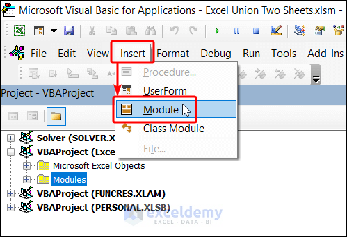
As a consequence, Module1 will be a brand-new module.
Double-click Module1 after that, and then type the following VBA code into the editor.

Sub Union_Two_Sheets()
Dim ws() As Variant
ws = Array("November", "December")
Result_Sheet = "Union Sheets Using VBA"
Union_Gap = 1
Set Result_Cell = Worksheets(ws(0)).UsedRange.Cells(1, 1)
First_Row = Result_Cell.Row
First_Column = Result_Cell.Column
For i = LBound(ws) To UBound(ws)
    Worksheets(ws(i)).Activate
    Row_Width = ActiveSheet.UsedRange.Columns.Count
    ActiveSheet.UsedRange.Copy
    Worksheets(Result_Sheet).Activate
    ActiveSheet.Cells(First_Row, First_Column).PasteSpecial Paste:=xlPasteAll
    First_Column = First_Column + Row_Width + Union_Gap
Next i
Application.CutCopyMode = False
End Sub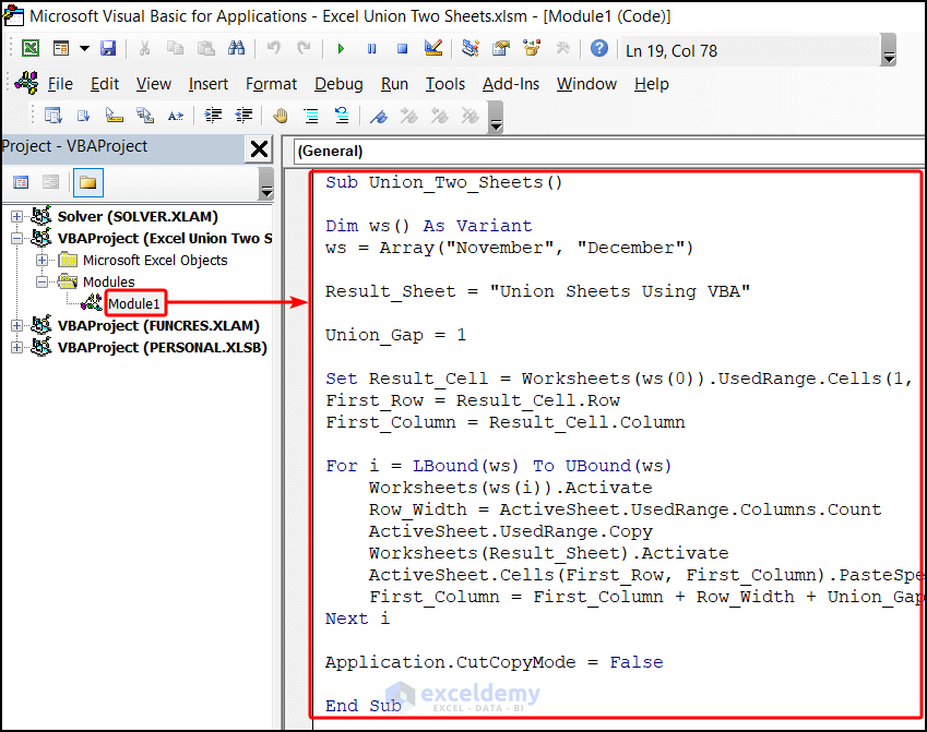

Now, press the Run button.

After pressing the Run button, the result looks like the following image. Two datasets from two different worksheets have been placed side by side using a VBA code.

Note:

Here, you have to edit your target sheet name in the Result_Sheet variable. And, you have to put your desired sheet names that you want to merge in the ws variable in the code.

Conclusion

Follow these steps and stages on Excel Union Two Sheets. You are welcome to download the workbook and use it for your own practice. If you have any questions, concerns, or suggestions, please leave them in the comments section of our blog ExcelDemy.