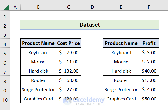
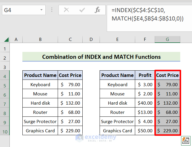
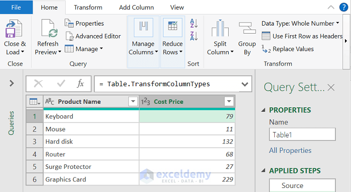
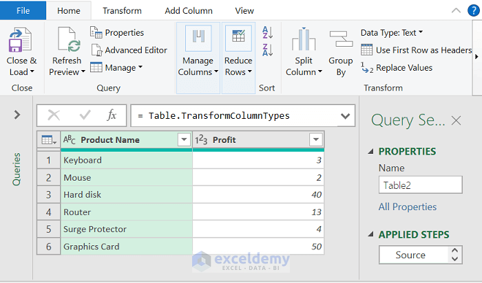
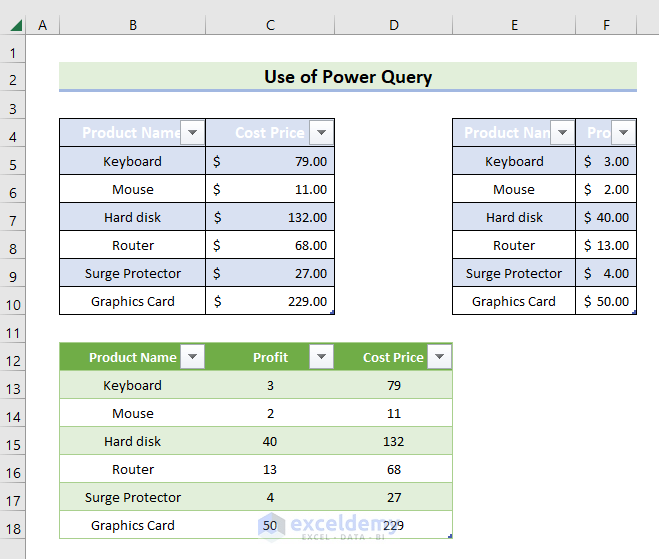
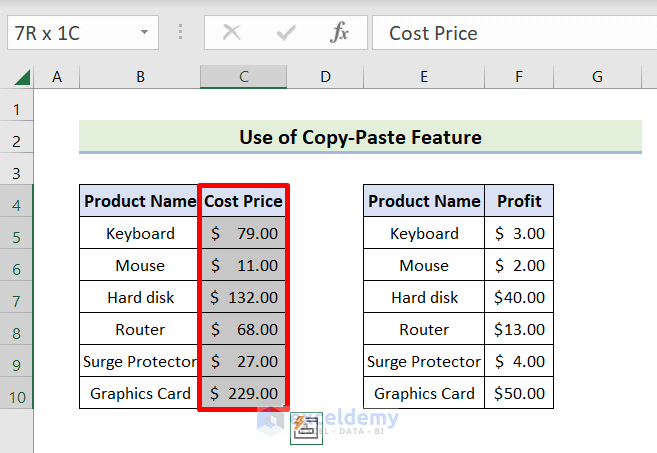
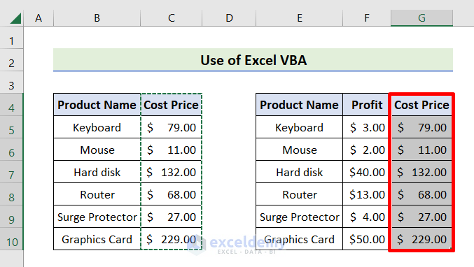
The left table contains two columns titled Product Name and Cost Price. The right side holds the Product Name column and a column named Profit.
Method 1 – Utilizing the Excel VLOOKUP Function to Join Two Tables
STEPS:
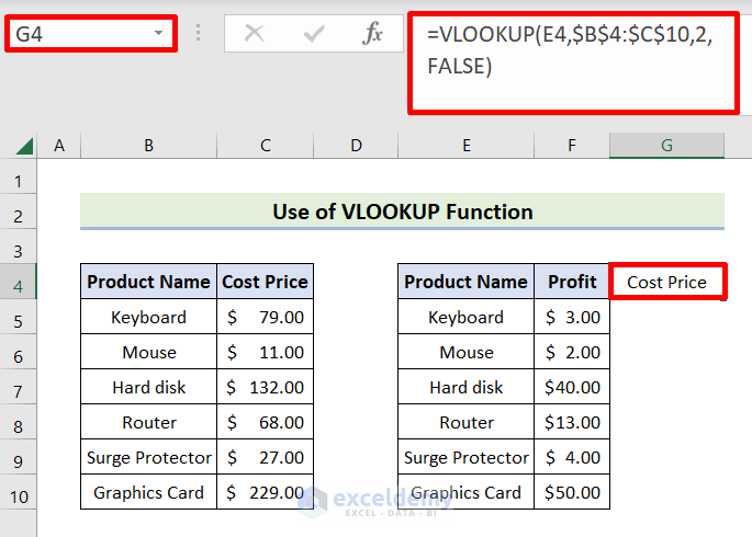
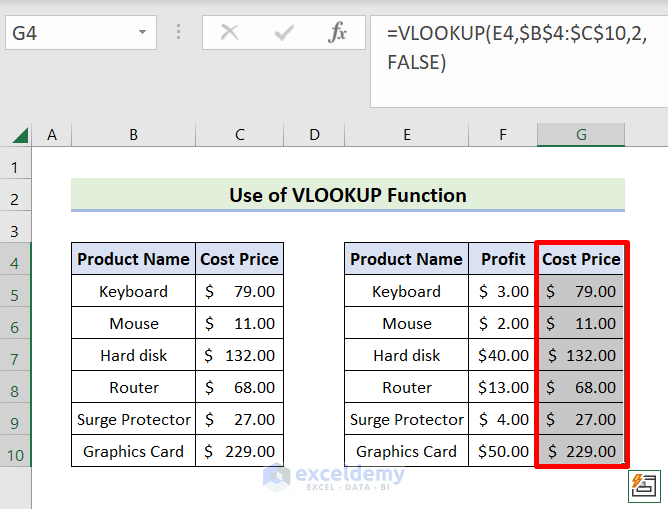
- Select the G4 cell.
- Input the following formula in G4.
=VLOOKUP(E4,$B$4:$C$10,2,FALSE)
- Hit the Enter or Tab key.
- You’ll see the outcome below.
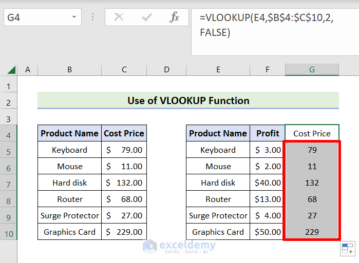
- You need to apply the same formula for the subsequent cells.
- Hold the Fill Handle icon and move it to G10.
- Select the C4:C10 range.
- Go to the Home tab.
- From the Clipboard group, click the Format Painter icon.
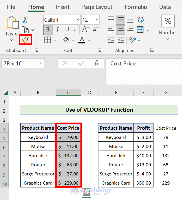
- A brush cursor will appear. Click the G4 cell.
- The desired output will be displayed.
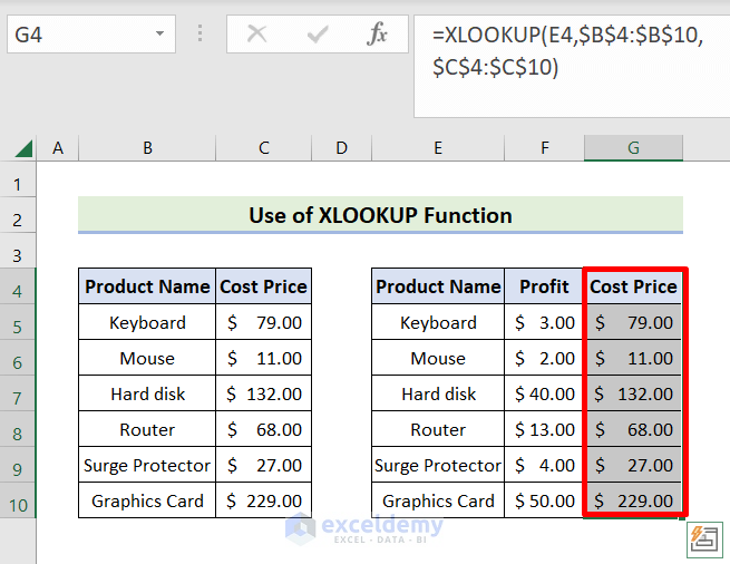
Method 2 – Creating a Union of Tables with the XLOOKUP Function
STEPS:
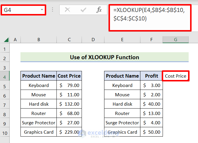
- Choose the G4 cell.
- Insert the following formula in G4.
=XLOOKUP(E4,$B$4:$B$10,$C$4:$C$10)
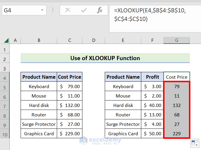
- Press Enter or Tab keys.
- You will see the outcome below.
- You need to apply the same formula for the subsequent cells.
- Hold the Fill Handle icon and move it to G10.
- Select the C4:C10 range.
- Navigate to the Home tab.
- Within the Clipboard group, select the Format Painter symbol.
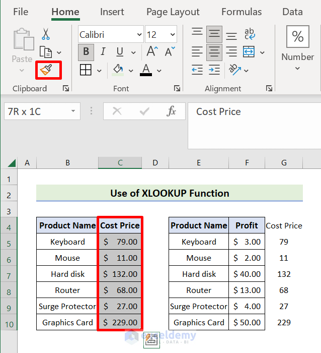
- A brush cursor will appear, then click the G4 cell.
- Produce the intended result.
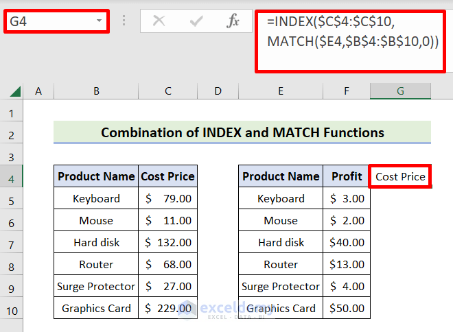
Method 3 – Combining INDEX and MATCH Functions to Merge Tables
STEPS:
- Select the G4 cell.
- Use the following formula in cell G4:
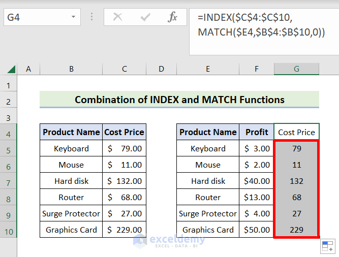
=INDEX($C$4:$C$10,MATCH($E4,$B$4:$B$10,0))
- Press Enter or Tab to continue.
- Drag the Fill Handle symbol to G10.
- Select the C4:C10 range for the time being.
- Navigate to the Home tab next.
- From the Clipboard group, choose the Format Painter symbol.
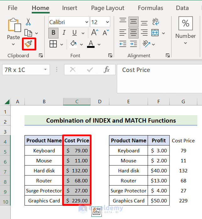
- Click the G4 cell with the resulting brush-shaped cursor.
- You will achieve the desired outcome.
Method 4 – Applying Excel Power Query to Combine Two Tables
STEPS:
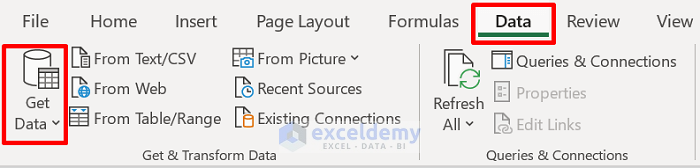
- Navigate to the Data tab.
- Choose Get Data from the Get & Transform Data group.
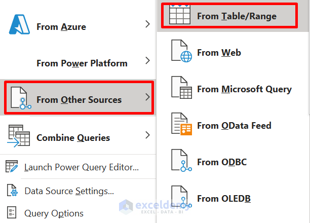
- Select the From Other Sources option and pick Form Table/Range.
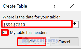
- The Create Table window will open.
- Type the range for the left table in the input box.
- Check My Table Has Headers and hit OK.
- The Power Query Editor window will open to display the left table as Table1.
- Close the Power Query Editor window.
- Tap the Keep button.

- The table will be stored in a new sheet titled Table1 in this case.
- Follow the same procedures to create the table on the right side.
- The Power Query Editor window will show the right table as Table2.
- Select the Combine group, click the little Down Arrow icon, and pick Merge Queries.
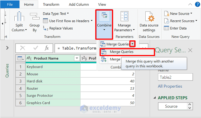
- The Merge window will display.
- Select the Product Name column from both Table1 and Table2.
- Pick the Left Outer from the Join Kind section and hit OK.

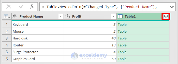
- Two tables will join and display, as shown below.
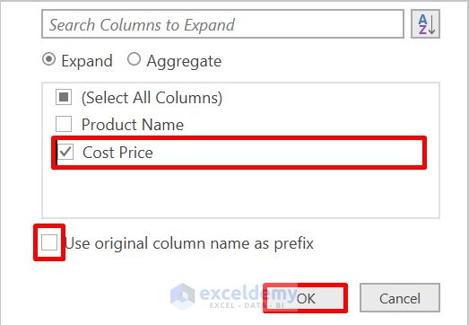
- Click the Expand icon.
- Check the Cost Price column and uncheck the Prefix option.
- Click OK.
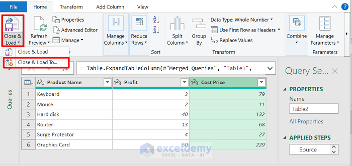
- From the Power Query Editor window, choose Close & Load, followed by Close & Load To.
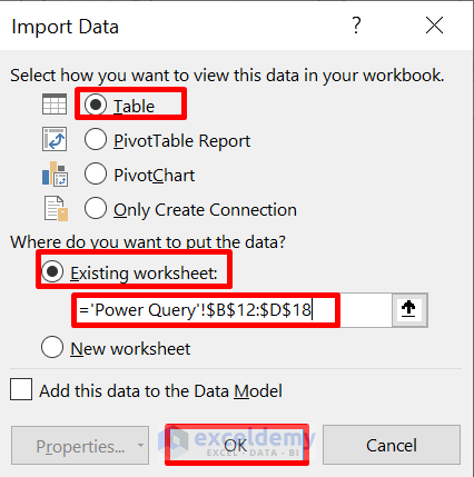
- The Import Data window will appear.
- Check the Table option and the Existing Worksheet field.
- Type the Sheet Name with an Exclamation mark followed by the range and hit OK.
- It will produce the desired output below.
Method 5 – Using Copy-Paste to Merge Tables
STEPS:
- Select the C4:C10 range.
- Tap Ctrl + C.
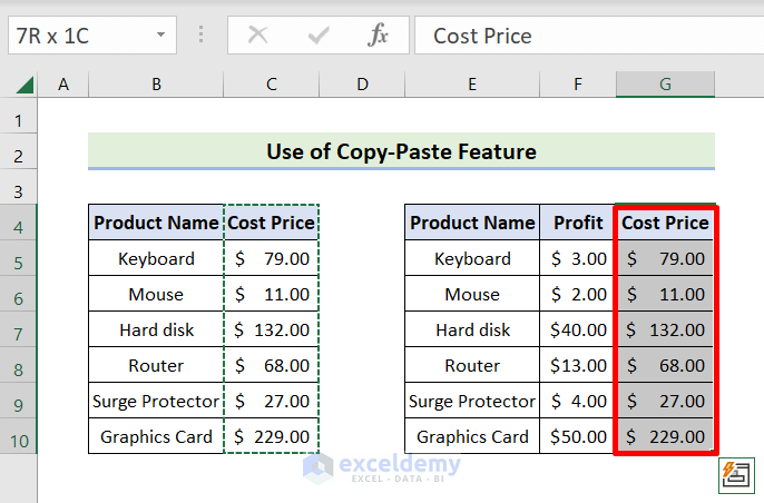
- Mark another column, in this case, G4:G10.
- Press Ctrl + V.
- You will obtain the intended output below.
Method 6 – Joining Two Tables Through Excel VBA
STEPS:
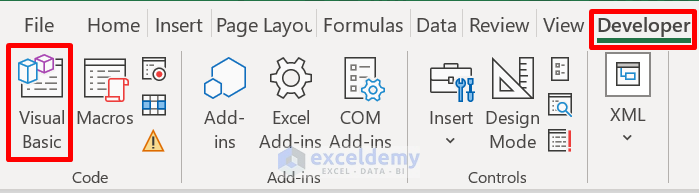
- Navigate to Developer.
- Choose Visual Basic.
- Click Insert, then Module.
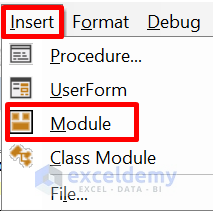
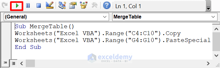
- Insert the code below into the Module Box.
Sub MergeTable()
Worksheets("Excel VBA").Range("C4:C10").Copy
Worksheets("Excel VBA").Range("G4:G10").PasteSpecial
End Sub- Press F5 or select the Run symbol.
- It will provide the desired output below.
Download the Practice Workbook
Related Articles
<< Go Back to Excel Union | Excel Operators | Excel Formulas | Learn Excel
Get FREE Advanced Excel Exercises with Solutions!
