In this article, we will explain how to perform a Union query in Excel to merge multiple tables with one common column or row.
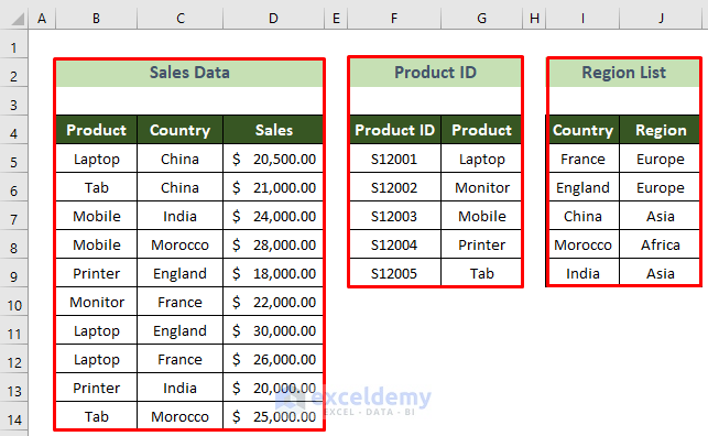
Suppose we have 3 individual datasets – Sales Data, Product ID, and Region List, which are related to each other. Let’s perform a Union query to merge them into one table.
Step 1 – Collect Data and Create a New Query Connection
First we’ll prepare the datasets into tables and create connections.
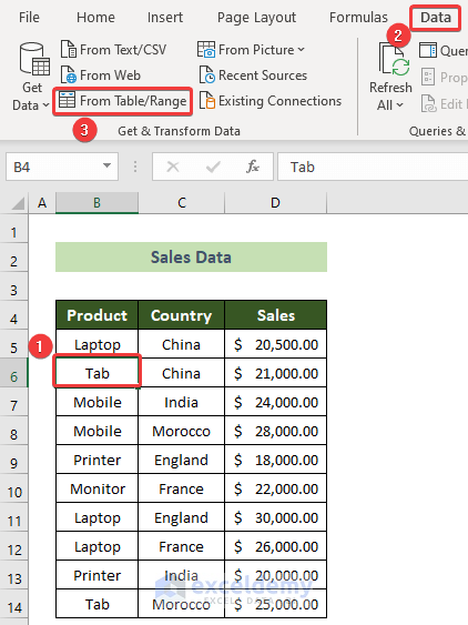
- Click on any cell inside the dataset.
- Go to the Data tab >> From Table/Range tool.
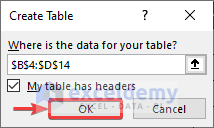
- In the Create Table window that opens, click on OK.
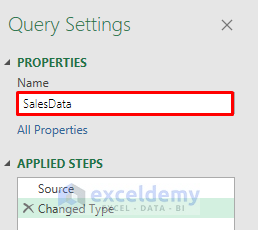
The Power Query Editor window will open.
- In the Query Settings pane, under the Properties group, enter the table’s name (SalesData here) in the Name text box.
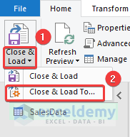
- Under the File tab, click on the Close & Load arrow and select the option Close & Load To…
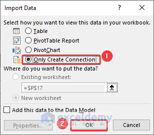
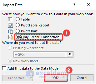
The Import Data window will appear.
- Choose the Only Create Connection option and click on OK.
The SalesData table is prepared for merging.
- Follow similar procedures for all the other datasets to prepare them for the Union query.
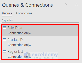
The following will be visible on the right side of your Excel file in the Queries & Connections window.
Read More: How to Create Union of Two Tables in Excel
Step 2 – Prepare to Combine the Queries
Now we are ready to perform a Union query between these tables.
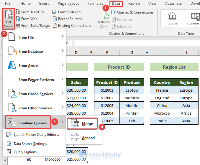
- Go to the Data tab >> Get Data tool >> Combine Queries option >> Merge option.
The Merge window will appear.
Step 3 – Make the Necessary Selections in the Merge Window
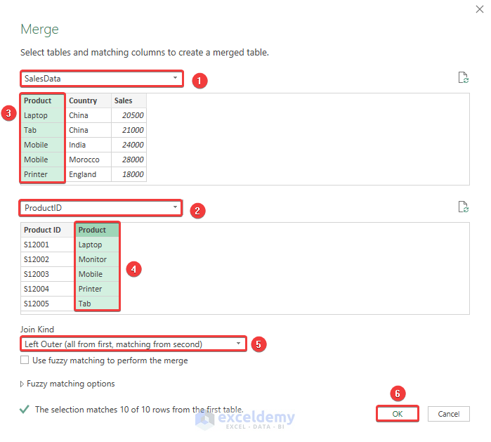
Now we’ll perform a Union query between the SalesData table and the ProductID table.
- In the first Preview window choose the SalesData table, and in the second Preview window choose the ProductID table.
- Click on the common column (Product) in both tables.
- Choose Left Outer for the Join Kind and click on OK.
Read More: How to Do Union of Two Columns in Excel
Step 4 – Place the Values Properly
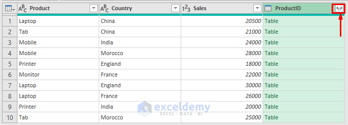
As a result the merge will take place, but the values haven’t been placed properly.
- Click on the double arrow button inside the ProductID header.
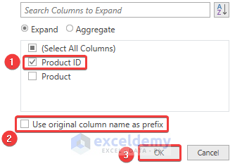
- From the drop-down list that opens, tick the Product ID option only, untick the Use original column name as prefix, and click on OK.
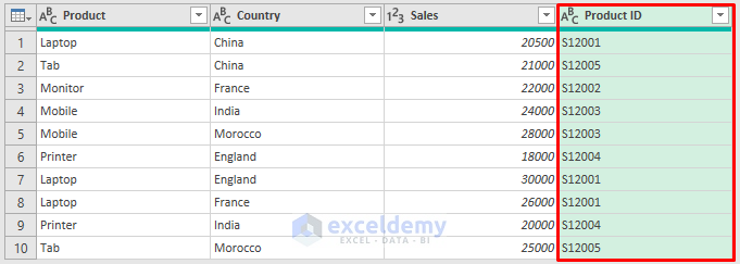
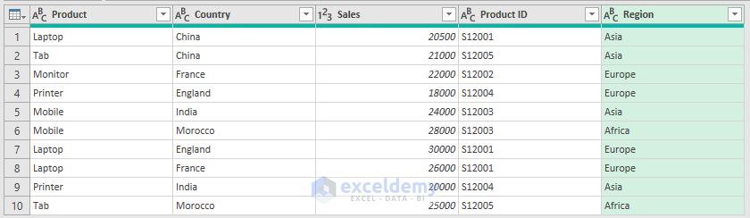
The two tables are merged properly now.
Step 5 – Create Another Connection
- As we need to merge another table, go to the File tab >> Close & Load arrow >> Close & Load To… option.

The Import Data window will appear.
- Click on the Only Create Connection option and click on OK.
We can now import the merged table as the Merge1 table.
Step 6 – Make the Necessary Selections in the Merge Window (Same as the Step 3)
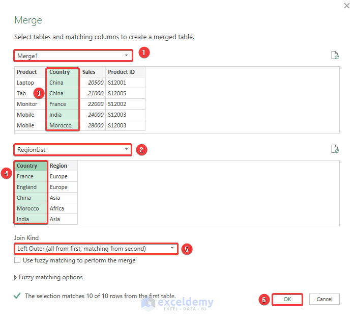
We’ll repeat the merging procedures above to merge this Merge1 table and the RegionList table.
- In the first Preview window choose the Merge1 table, and in the second Preview window choose the RegionList table.
- Click on the Country column in both tables.
- Choose Left Outer as the Join Kind and click on OK.
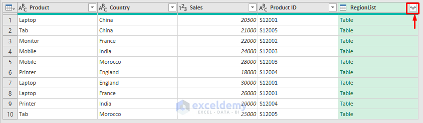
The RegionList column will also be merged into the previously merged table.
- For proper values, click on the double arrow button on the RegionList header.
- From the drop-down list that appears, tick on the Region option only and untick the option Use original column name as prefix.
- Click on OK.
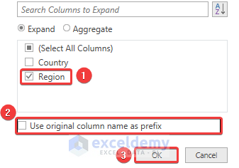
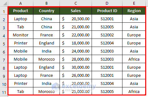
We have proper values in the Region column.
Last Step – Close and Load the Data
- Under the File tab, click on the Close & Load button.

We have completed merging all three tables with a Union query in Excel.
Download Practice Workbook
Related Article
<< Go Back to Excel Union | Excel Operators | Excel Formulas | Learn Excel
Get FREE Advanced Excel Exercises with Solutions!
