This is an overview.
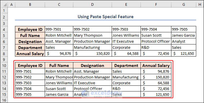
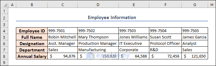
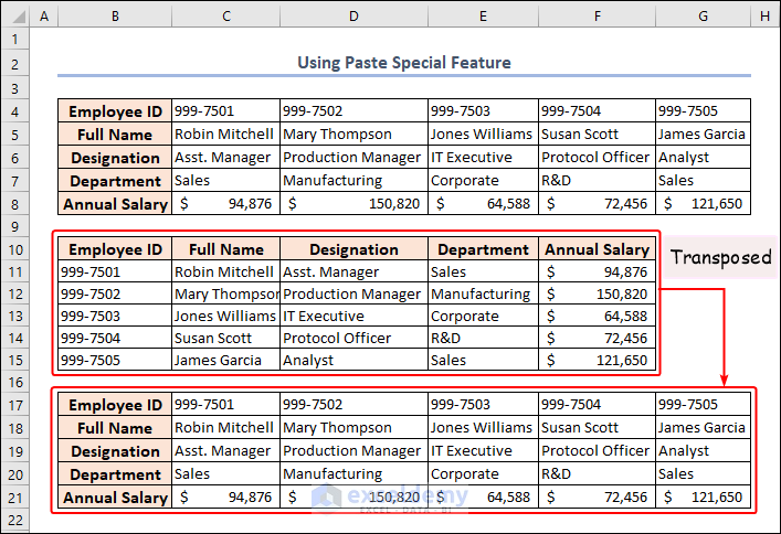
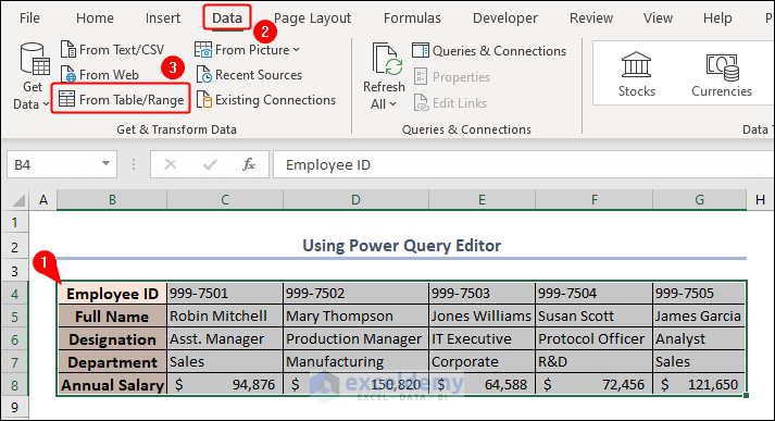
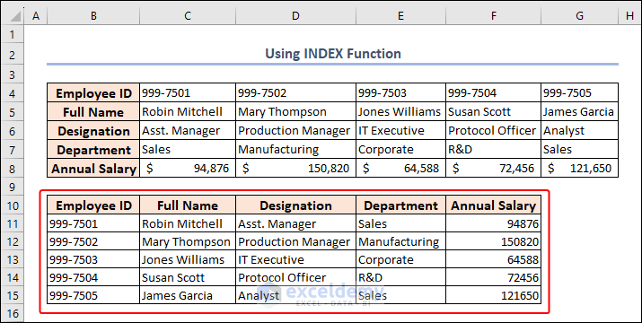
This dataset includes Employee Information: ID, Full Name, Designation, Department, and Annual Salary.
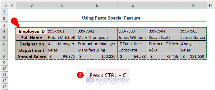
Method 1 – Using the Paste Special Feature to Swap Columns and Rows
- Select the entire dataset (B4:G8) and press CTRL + C to copy the range.
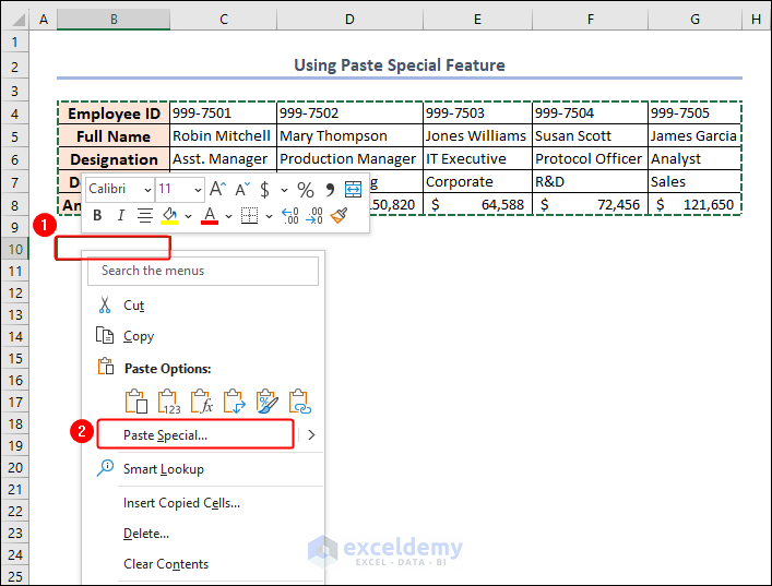
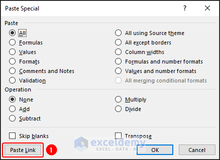
- In the Paste Special dialog box, check Transpose and click OK.

This is the output.

- Follow the same steps to reverse the result:
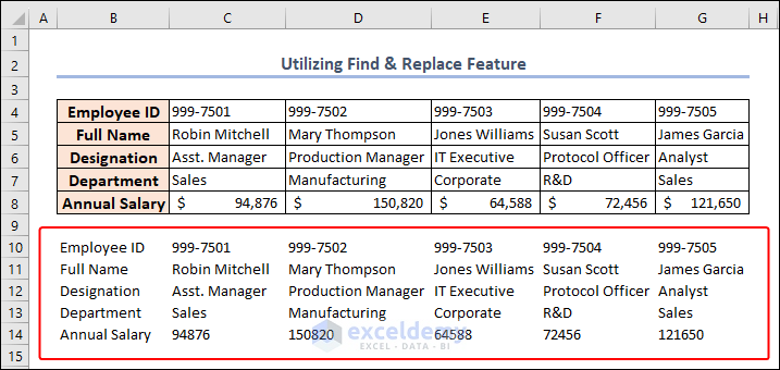
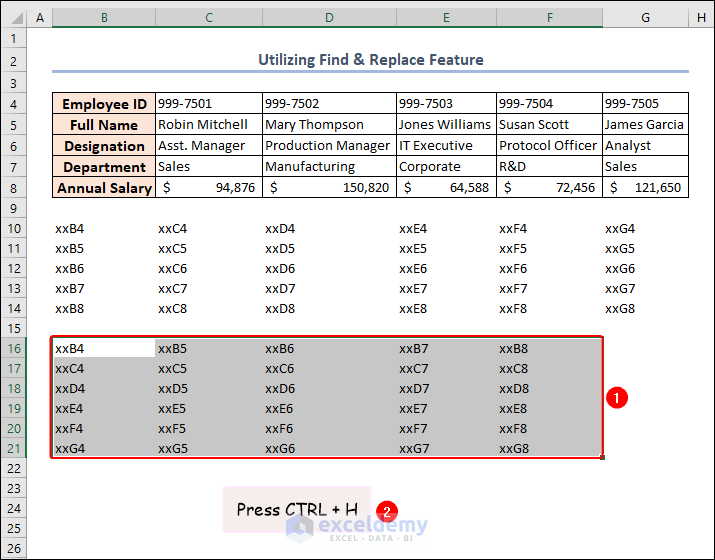
Method 2 – Utilizing the Find & Replace Feature to Make Swapping Dynamic
- Select the entire dataset and copy it.
- Open the Paste Special dialog box following the steps in Method 1.
- Click Paste Link.
It’ll paste the data without formatting in the selected output range.
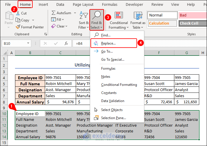
- Select the pasted range (B10:G14) and go to the Home tab.
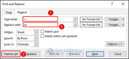
- Select Find & Replace >> Replace. You can also press CTRL + H.
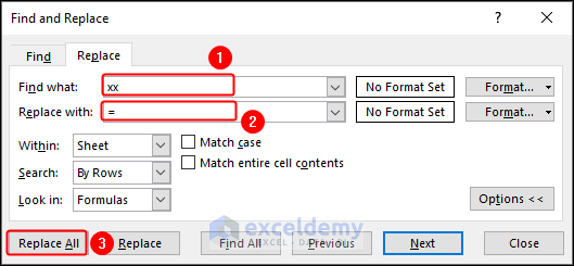
- In the Find and Replace dialog box, enter = and xx in Find what and Replace with.
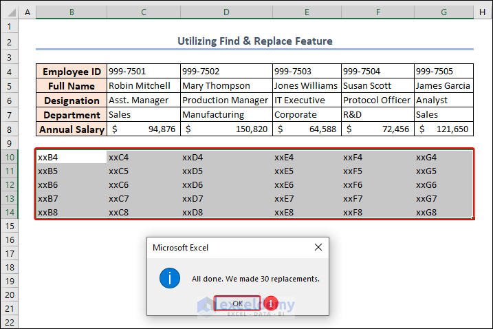
- Click Replace All.
The message “All done. We made 30 replacements.” is displayed. xx replaced “=”.
- Click OK.
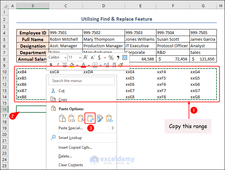
- Copy B10:G14 and paste it in B16.
- Right-click.
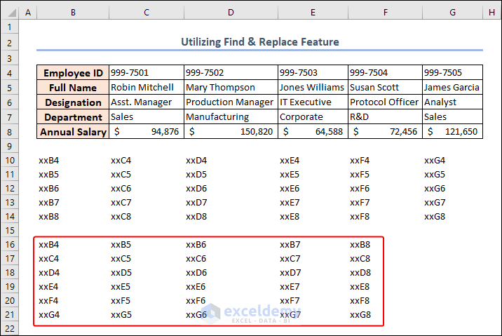
- Select Transpose (T) in Paste Options.
This is the output.
- Select the pasted range and press CTRL + H to open the Find and Replace dialog box.
- Enter xx and = in Find what and Replace with.
- Click Replace All.
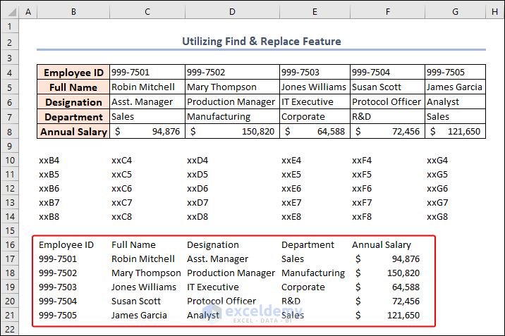
This is the output.
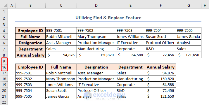
This is the output (after formatting and hiding rows).
Method 3 – Swapping Columns and Rows in Large Datasets Using the Power Query Editor
- Select the dataset and go to Data >> From Table/Range.
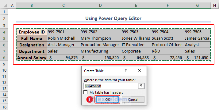
In the Create Table dialog box, the selected table range is displayed.
- Click OK.
- In the Power Query Editor window, select Transform >> Transpose in Table.
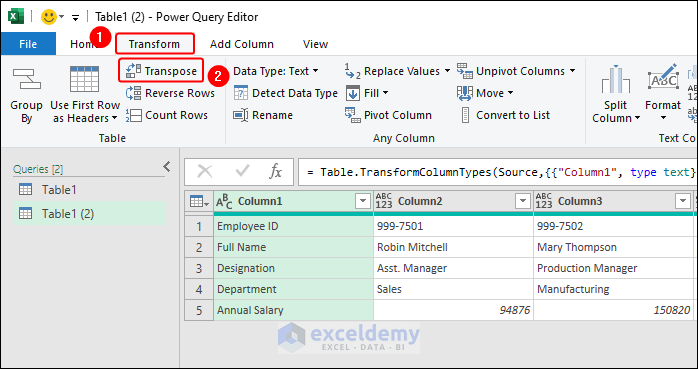
The table is transposed.
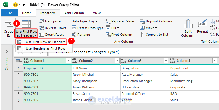
- Select Use First Row as Headers.
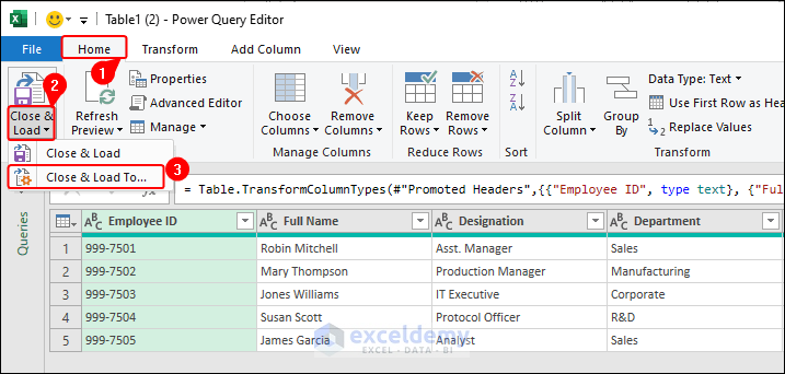
- In the Home tab, click Close & Load >> Close & Load To… .
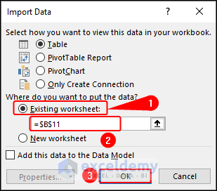
- In the Import Data dialog box, choose the output destination. Here, Existing worksheet and B11 as cell reference.
- Click OK.
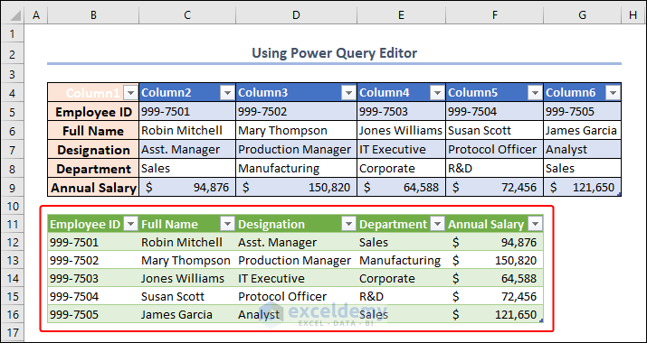
This is the output.
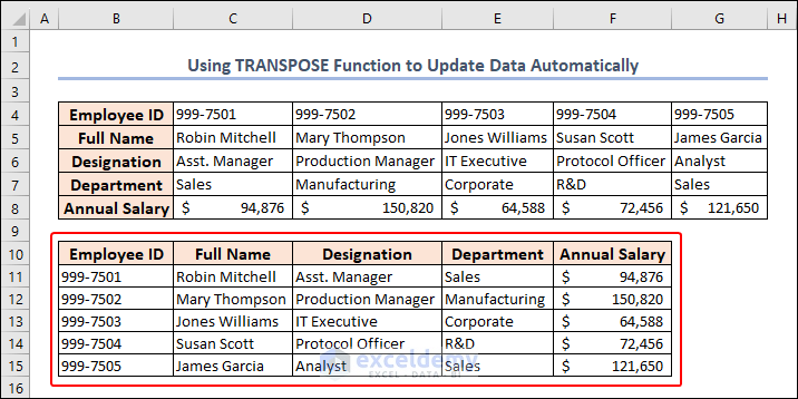
Method 4 – Using the TRANSPOSE Function to Update Data Automatically
- In B10, use the following formula and press ENTER.
=TRANSPOSE(B4:G8)As it’s an array formula, it returns an array containing the transposed data without formatting.
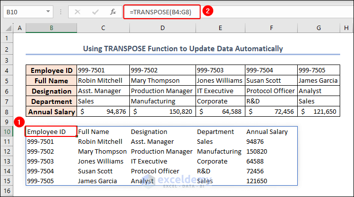
This is the output (after formatting).
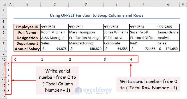
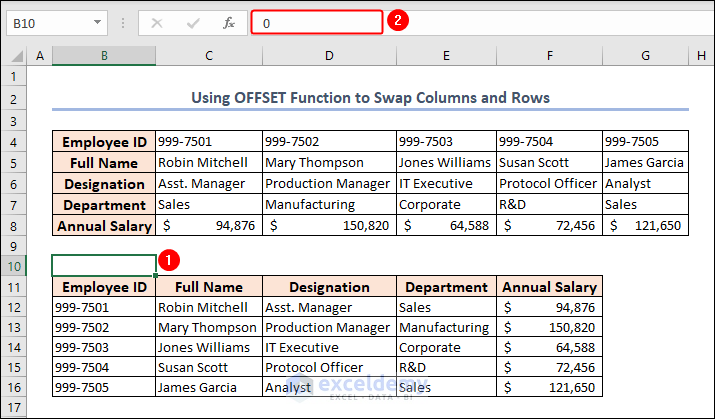
Method 5 – Swapping Columns and Rows using the OFFSET Function
- Enter serial numbers from 0 to the (total row number-1) or (5 – 1) or 4 (there are 5 rows) in an area to paste the data; enter serial numbers from 0 to the (total column number-1) or (6 – 1) or 5 (there are 6 columns) in the left of the that area.
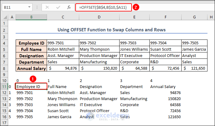
- Use the following formula in B11 and press ENTER.
=OFFSET($B$4,B$10,$A11)- Drag down the Fill Handle to copy the formula to the other cells.
- Apply formatting.
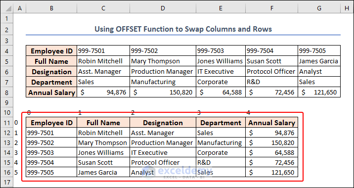
- Select B10. The formula bar shows 0, but it isn’t visible in the worksheet cell.
You can hide extra numbers around the output cells by changing their font color to white.
Method 6 – Use the VLOOKUP Function
- Transpose the first column and first row manually and enter the values in the first row and first column of the output range.
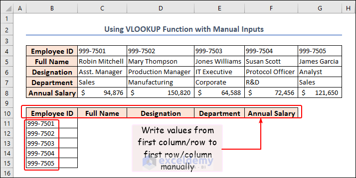
- In C11, use the following formula and press ENTER.
=VLOOKUP($B11,TRANSPOSE($C$4:$G$8),COLUMN()-1,FALSE)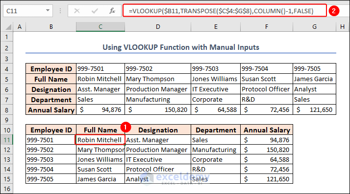
This is the output.
Method 7 – Swap Columns and Rows Using the INDEX Function
- Enter the following formula in B10 and press ENTER.
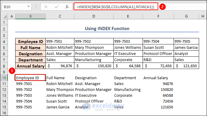
=INDEX($B$4:$G$8,COLUMN(B2),ROW(B2))This is the output (after formatting).
Method 8 – Combine the INDIRECT and the ADDRESS Functions to Swap Columns and Rows
- Use the following formula in B10.
- Drag down the Fill Handle to see the result in the rest of the cells.
=INDIRECT(ADDRESS(COLUMN(C5)-COLUMN($B$4)+ROW($B$4), ROW(C5)-ROW($B$4)+COLUMN($B$4)))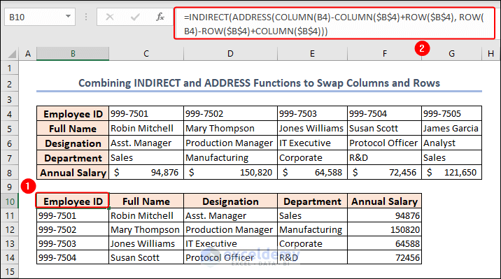
Formula Breakdown
- COLUMN(C5): returns the column number of C5.
- COLUMN($B$4): returns the column number of B4. The dollar signs around the row and column reference indicate an absolute reference (the reference will not change if the formula is copied to other cells).
- COLUMN(C5)-COLUMN($B$4): calculates the number of columns between the reference cell (B4) and the target cell (C5).
- ROW($B$4): returns the row number B4.
- ROW(C5)-ROW($B$4): calculates the number of rows between the reference cell (B4) and the target cell (C5).
- COLUMN(C5)-COLUMN($B$4)+ROW($B$4): adds the number of columns and rows calculated in steps 3 and 4 to the row number in the reference cell.
- ROW(C5)-ROW($B$4)+COLUMN($B$4): adds the number of rows and columns calculated in step 5 to the column number in the reference cell.
- ADDRESS(COLUMN(C5)-COLUMN($B$4)+ROW($B$4), ROW(C5)-ROW($B$4)+COLUMN($B$4)): takes the row and column values calculated in steps 6 and 7 and returns the cell address as a text string.
- INDIRECT(ADDRESS(COLUMN(C5)-COLUMN($B$4)+ROW($B$4), ROW(C5)-ROW($B$4)+COLUMN($B$4))): converts the text string returned by the ADDRESS function into a reference to the target cell. The INDIRECT function references a cell based on a text string.
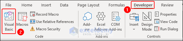
Method 9 – Applying a VBA Code to Swap Columns and Rows in Large Datasets in Excel
- Go to the Developer tab and click Visual Basic in Code.
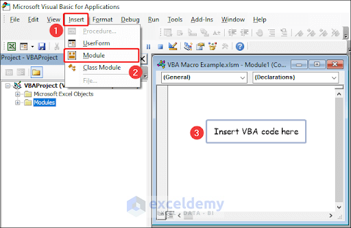
In the Microsoft Visual Basic for Applications window:
- Select Insert and choose Module.
- Enter the VBA code.
Sub Swap_Columns_Rows()

Dim inputRange As Range
Dim outputCell As Range
Dim outputRange As Range

'Get input range
Set inputRange = Application.InputBox("Select the range to transpose:", Type:=8)

'Get output cell
Set outputCell = Application.InputBox("Select the first cell of the output range:", Type:=8)

'Transpose data and copy formatting
Set outputRange = outputCell.Resize(inputRange.Columns.Count, inputRange.Rows.Count)
inputRange.Copy
outputRange.PasteSpecial Transpose:=True
inputRange.Copy
outputRange.PasteSpecial Paste:=xlPasteFormats, Transpose:=True

End Sub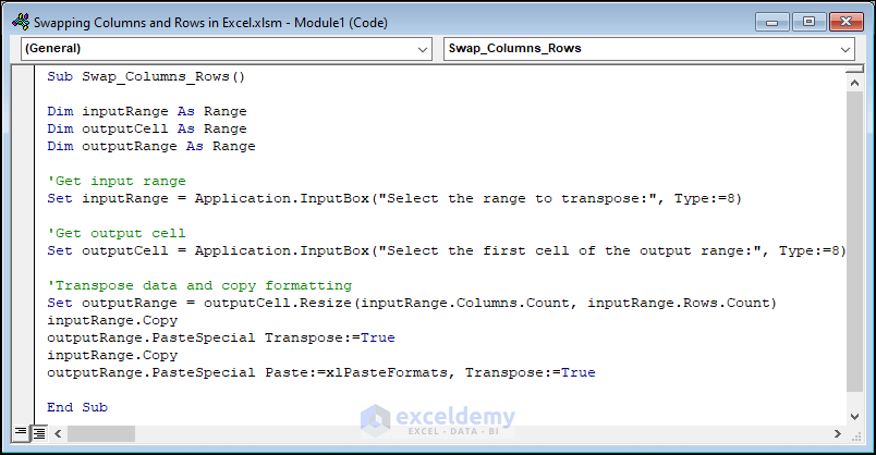
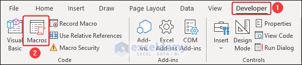
- To run the code, go to the Developer tab >> Macros in Code.
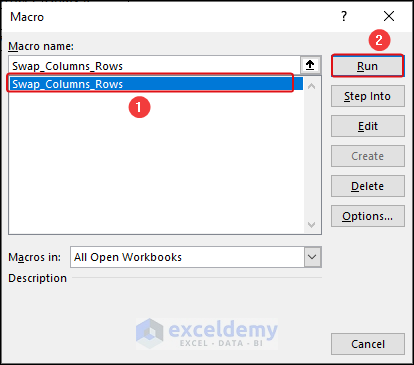
- Select the macro and click Run.
How to Switch Rows in Excel
To place Row 5 (Full Name) between rows 7 and 8.
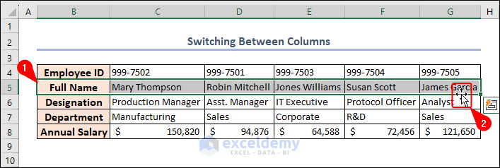
- Drag the cursor downwards until it reaches the top of Row 8. Press and hold SHIFTand release the row.
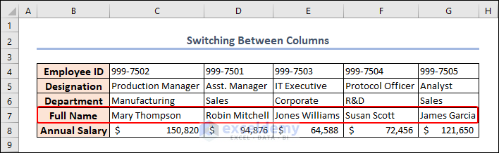
This is the output.
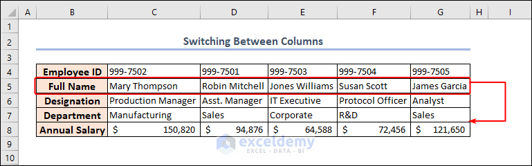
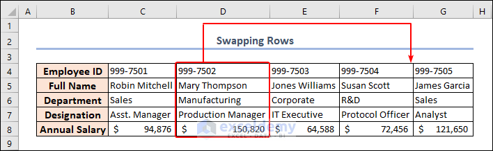
How to Swap Columns in Excel
To place Column D between columns F and G, follow the steps described in the previous section.
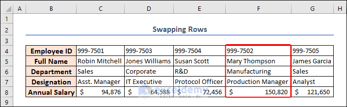
This is the output.
Download Practice Workbook
Download the following practice workbook.
Related Article
<< Go Back to Excel Cells | Learn Excel
Get FREE Advanced Excel Exercises with Solutions!
