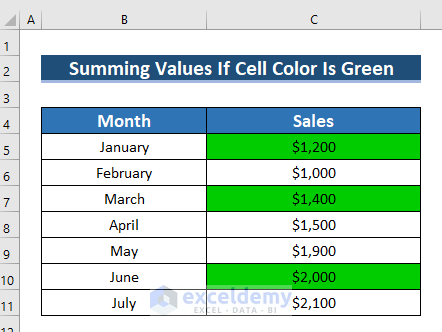
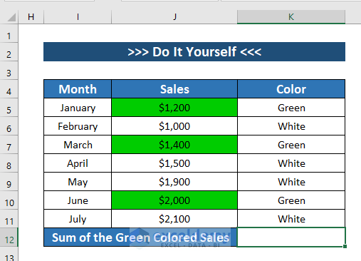
The following dataset has Month and Sales columns. The Sales column has several cells colored Green. Using this dataset, we will find the sum of the cells colored green.
Method 1 – Applying the SUMIF Function Using a Helper Column with Color Names Written Manually
Steps:
- Enter the following formula in cell C12:
=SUMIF(D5:D11,"Green",C5:C11)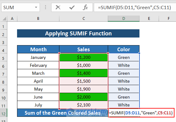
Formula Breakdown:
- SUMIF(D5:D11, “Green”, C5:C11) → the SUMIF function finds the sum of a range of cells based on specified criteria.
- D5:D11 → is the range.
- Green → is the criteria.
- C5:C11 → is the sum_range.
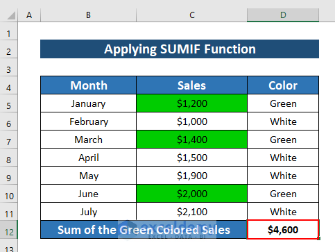
Output: $4600
- Press ENTER.
- The result is in cell C12.
Read More: How to Use If Statement Based on Cell Color in Excel
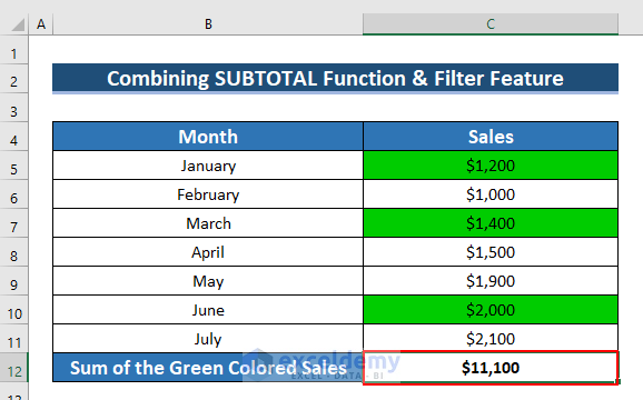
Method 2 – Using the SUBTOTAL Function and Applying the Filter Command to Filter Out Green Cells
Steps:
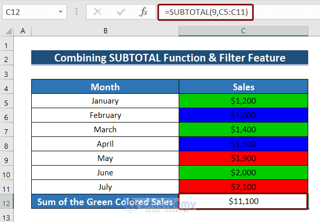
- Enter the following formula in cell C12:
=SUBTOTAL(9,C5:C11)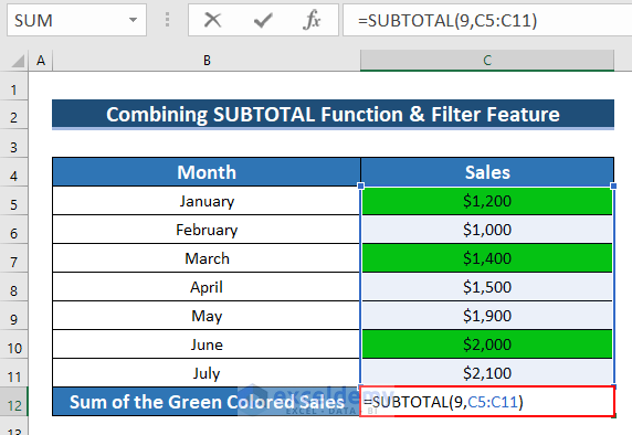
Formula Breakdown:
- SUBTOTAL(9, C5:C11) → the SUBTOTAL function finds out the subtotal in a range of cells.
- 9 → indicates the function_num.
- C5:C11 → is ref_1.
Output: $4600
- Press ENTER.
- The result is in cell C12.
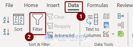
- To add the Filter icon to the column headings, we will select the column headings by selecting cells B4:C4.
- Go to the Data tab >> select Filter.
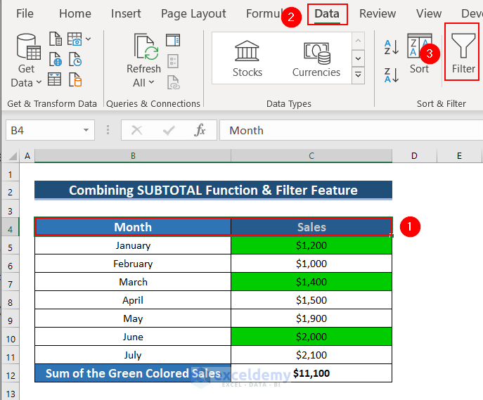
- The Filter icon is in the column headings.

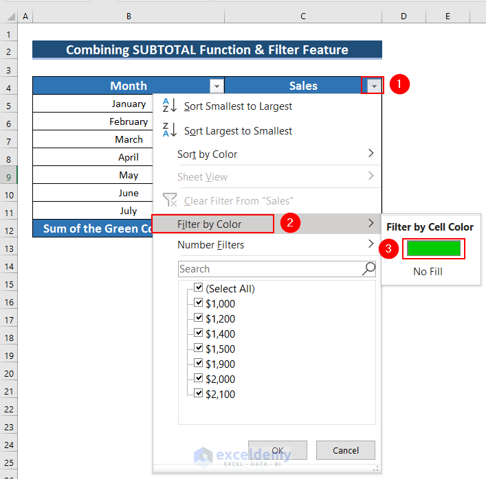
- Click on the Filter icon of the Sales >> select Filter by Color.
- Click on the color green.
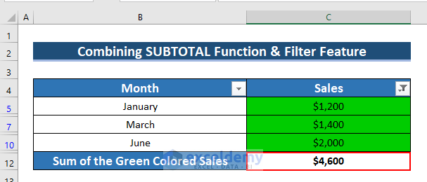
Here, you can insert a Table and use the Filter by Color to filter the Green color and find the sum of these green-colored cells.
- The Sum of the Green Colored Sales is in cell D12.
Read More: How to Use Conditional Formatting If Statement Is Another Cell
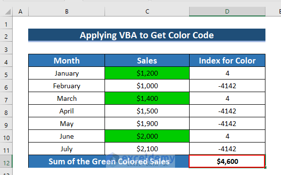
Method 3 – Using the GET.CELL Function to Get a Color Code for Green and Sum Using the SUMIF Function
Steps:
- Go to the Formulas tab >> select Name Manager.
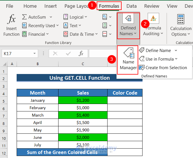
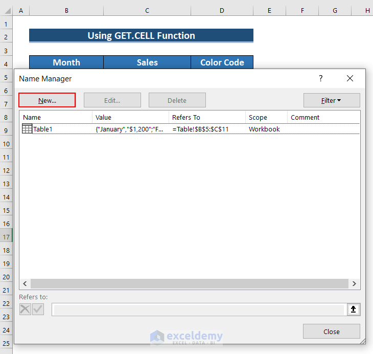
- A Name Manager dialog box will appear.
- Click on New.
- A Name dialog box will appear.
- In the Name box, enter color_code.
- In the Refers to box, enter the following formula:
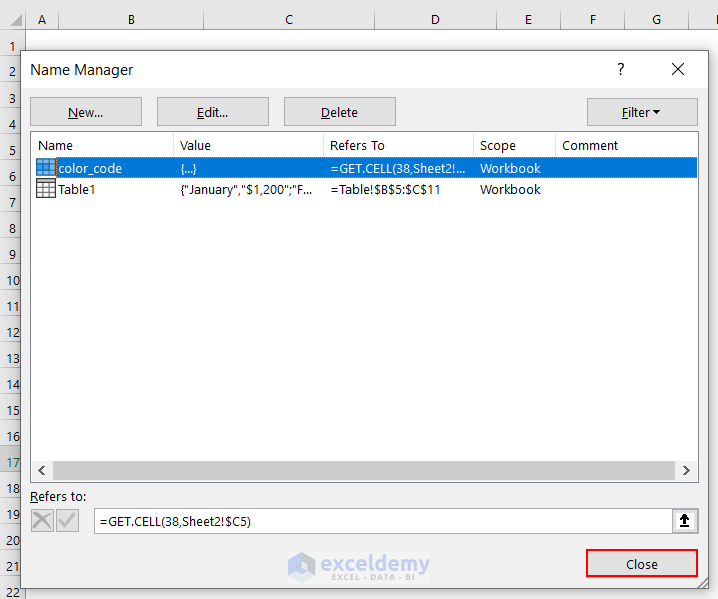
=GET.CELL(38, Sheet2!$C5)
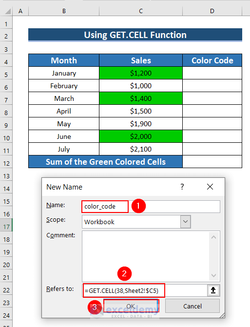
- Click Close.
- Enter the following formula in cell D5:
=color_code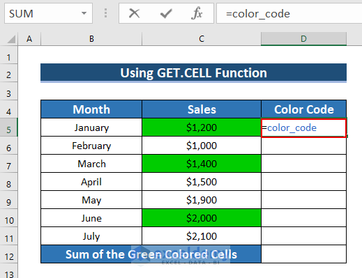
- Press ENTER.
- The result is in cell D5.
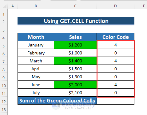
- Drag down the formula with the Fill Handle tool.
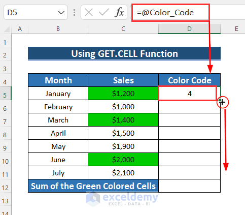
- The complete Color Code is in the column.
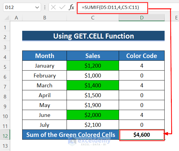
- Enter the following formula in cell D12:
=SUMIF(D5:D11,4,C5:C11)- Press ENTER.
- The result is in cell D12.
Read More: SUMIF vs SUMIFS in Excel
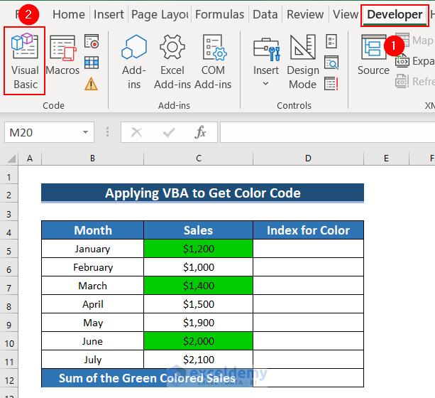
Method 4 – Using VBA Codes to Sum Green Cells Only
4.1. Get the Color Code with VBA and Then Apply the SUMIF Function to Get the Sum
Steps:
- Go to the Developer tab >> select Visual Basic.
- This will open a VBA Editor window. Press ALT+F11 to open the VBA Editor window.
- A VBA Editor window will open.
- From the Insert tab >> select Module.

- Enter the following code in the Module:
Function index_for_color(CellColor As Range)
   index_for_color = CellColor.Interior.ColorIndex
End Function
- Save the code >> go back to the Worksheet.
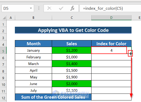
- Enter the following formula in cell D5:
=index_for_color(C5)
- Press ENTER.
- The index of the color Green is in cell D5.
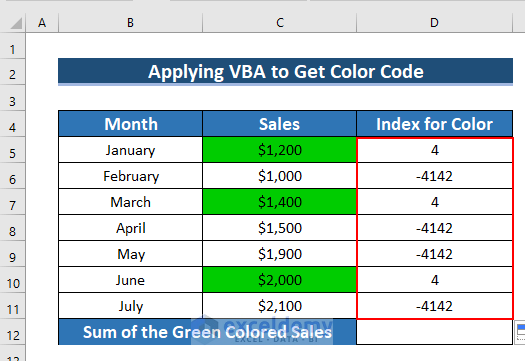
- Drag down the formula with the Fill Handle tool.
- The complete Index for Color is in the column.
- To find the Sum of the Green Colored Sales, enter the following formula in cell D12:
=SUMIF(D5:D11,4, C5:C11)
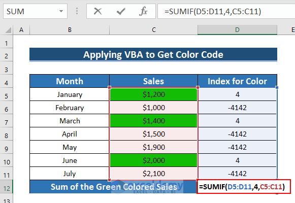
- Press ENTER.
- The result is in cell D12.
Read More: How to Use 3D SUMIF for Multiple Worksheets in Excel
4.2. Create a VBA Function to Get Added Value for a Selected Color (Green)
Steps:
- Follow the steps in 4.1 to open the Module.
- Enter the following code in the Module:
Function Sum_by_Green_Color(Cell_Color As Range, rRange As Range)
Dim c_sum As Double
Dim col_index As Integer
col_index = Cell_Color.Interior.ColorIndex
For Each cl In rRange
   If cl.Interior.ColorIndex = col_index Then
   c_sum = WorksheetFunction.Sum(cl, c_sum)
   End If
Next cl
Sum_by_Green_Color = c_sum
End Function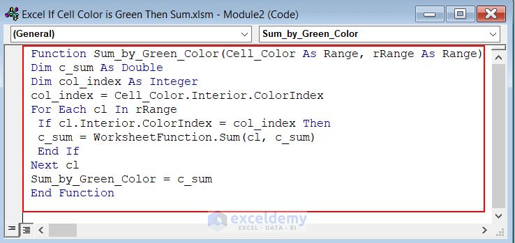
- Go back to our Worksheet.
- Enter the following formula in cell C13:
=Sum_by_Green_Color(C5,C5:C11)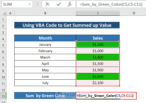
- Press ENTER.
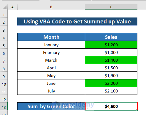
- The result is in cell C13.
Read More: How to Sum Colored Cells in Excel
Practice Section
You can download the Excel file and practice the explained methods.
Download the Practice Workbook
You can download the workbook to practice.
Related Articles
- Use If Then Else Statement in Excel VBA
- How to Ignore Blank Cells in Excel Sum
- Excel IF Statement Between Two Numbers
- How to Prepare IF Statement Contains Multiple Words in Excel
- Use Wildcard with If Statement in Excel
- How to Use IF Function with OR and AND Statement in Excel
- Use Multiple IF Statements in Excel Data Validation


Thanks for the tutorial, now how do I sum the cells if the cell color is green, blue, and red?
Hello ZHENG,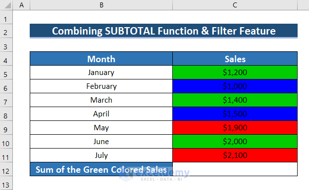
Thank you for taking the time to read our article. If you have cells of different colors (such as green, blue, and red) and want to sum them up, the easiest way is to use the SUBTOTAL function with the Filter command. For example, let’s say you have sales values in the range C5:C11, where cells C5, C7, and C10 are green, C6 and C8 are blue, and C9 and C11 are red.
1. To get the sum of a definite colored cell, insert the formula in a cell:
=SUBTOTAL(9,C5:C11)Here, the SUBTOTAL function inserted in cell C12 uses 9 as the “function_name” argument (which refers to the SUM function) and C5:C11 as “ref1”.
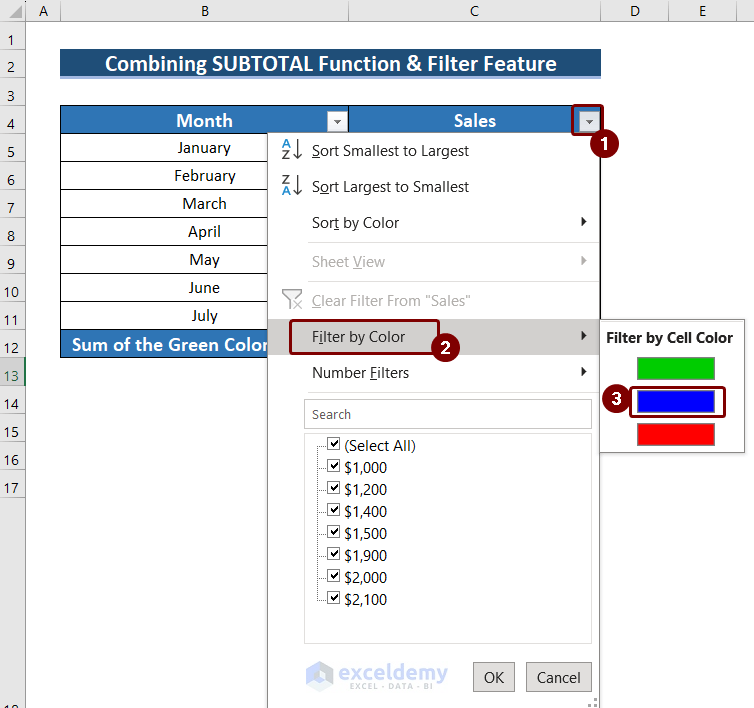
2. Select the column header and go to the Data tab > Sort & Filter > Filter.
3. Click on the Filter icon of the column and select “Filter by Color.” You will see three different colors to choose from.
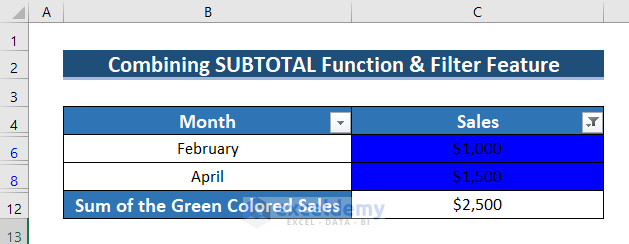
4. Select the color you want to sum up, and you will get the sum of all the cells with that color.
You can see the blue-colored cells filtered and summed up.
We hope this helps! Let us know if you have any further questions.
Regards,
Exceldemy Team