Most companies calculate work hours and overtime based on a 40 hour workweek (8 hours per day). In this article, we’ll calculate overtime based on the whole week, not based on an individual day. For example, if an employee worked 9 hours on Monday but his total hours for the week do not exceed 40, he will not be compensated for Monday’s overtime. Only when an employee exceeds 40 hours of work for a whole week will overtime compensation be due.
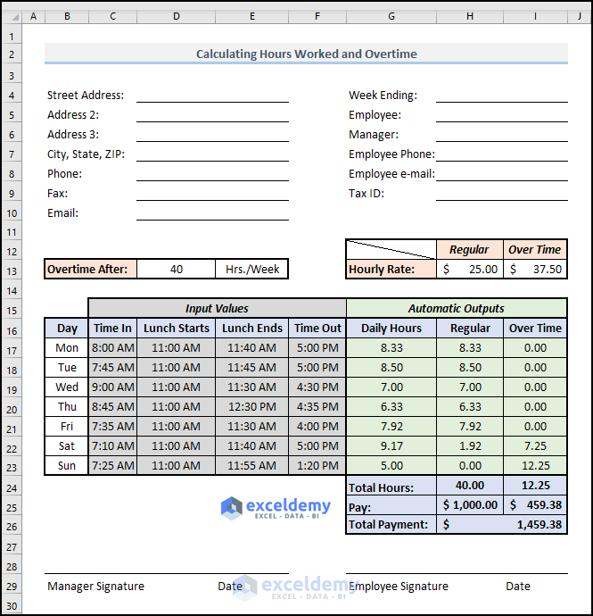
To demonstrate, we’ll create and fill the timesheet below.
We used the Microsoft Excel 365 version in this article, but you may use any other version at your convenience. If any steps don’t work in your version, please leave us a comment and let us know.
Step 1 – Create the Basic Outline
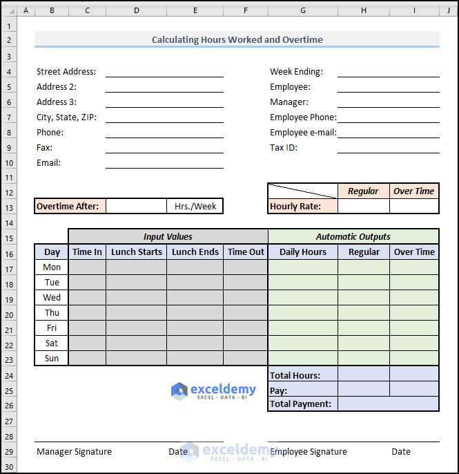
First let’s create a basic outline of the timesheet where we can insert all our necessary inputs and get the desired outputs.
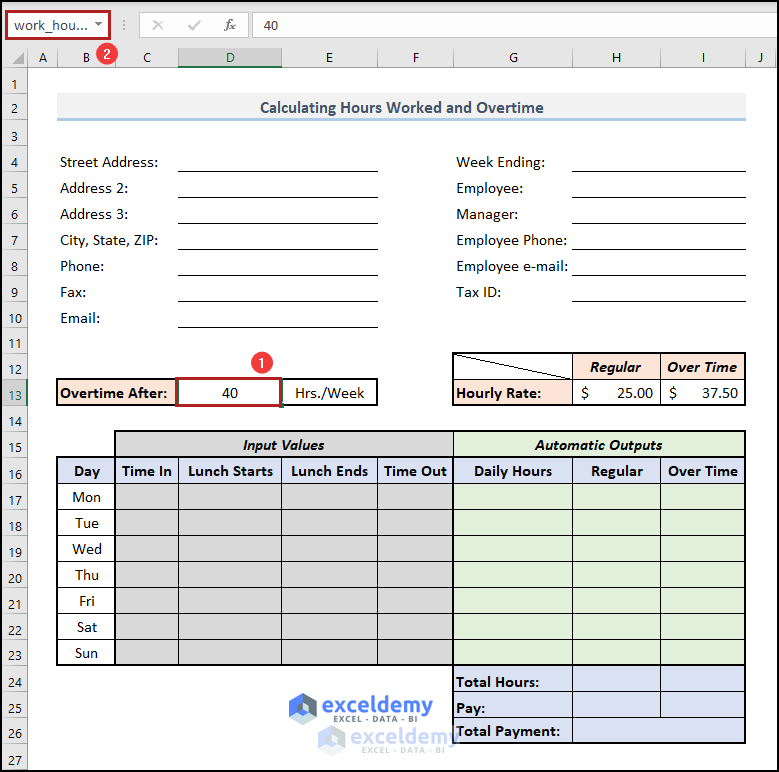
- Construct an enticing heading such as “Calculating Hours Worked and Overtime” in cell B2, and apply the Heading 2 cell style in that cell.
- Leave blank spaces in the B4:I10 range of cells for entry of the employee’s name and the employer’s information.
- Construct some tables in the B12:I26 range of cells as shown in the illustration below.
- Make a place for authorization in the B28:I29 range.
Step 2 – Set Weekly Work Hours and Pay Rate
Now let’s specify the regular and overtime hourly rates, and apply an Excel formula to calculate overtime based on these values.
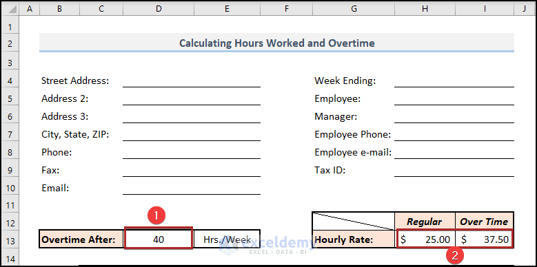
- In cell D13, enter 40 as the regular hours per week. Any value above 40 will be treated as overtime. If your office maintains different working hours per week, input that value in this field instead.
- Enter the Regular Hourly Rate in cell H13. Here, we used $25/hr.
- Enter the Overtime Hourly Rate, here $37.50/hr. Normally the general working hour rate is lower than the overtime hourly rate.
For the user’s convenience, let’s define names for some cell ranges.
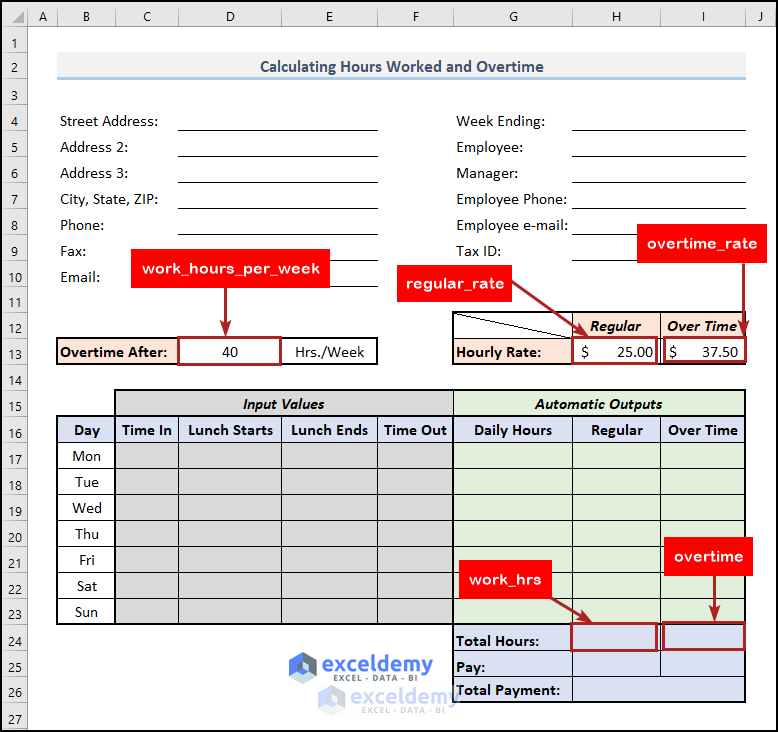
- Change the name of cell D13 to works_hours_per_week.
- Replace the names of cells H13 and I13 with regular_rate and overtime_rate respectively.
- In cells H24 and I24, change the names to work_hrs and overtime respectively.
Note: It’s not mandatory to change the cell name, but doing so helps the end users to understand the internal operation easily.
To define a new name for a cell:
- Select the cell (here, D13).
- In the small box at the top-left side of the display, enter your preferred name.
Step 3 – Enter Required Data
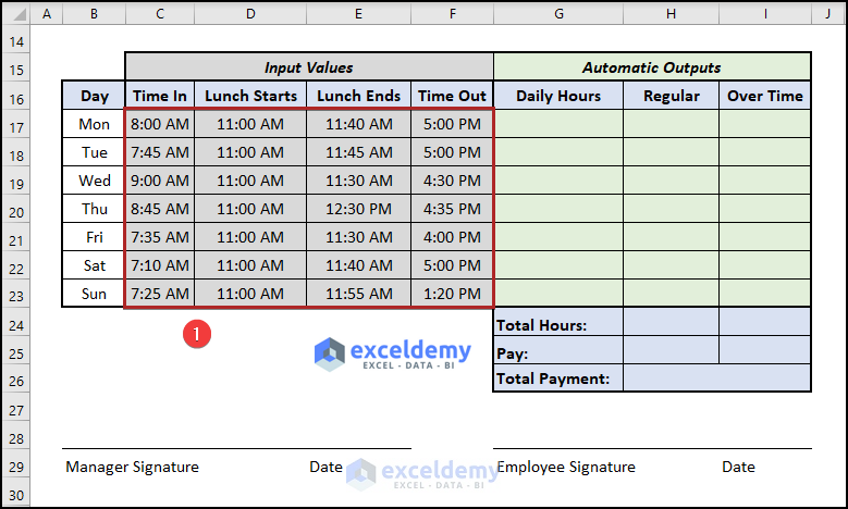
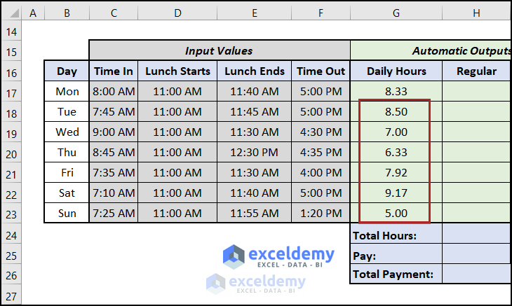
- Enter the necessary data like Time In, Lunch Starts, Lunch Ends, and Time Out in the sheet.
Step 4 – Calculate Daily Working Hours
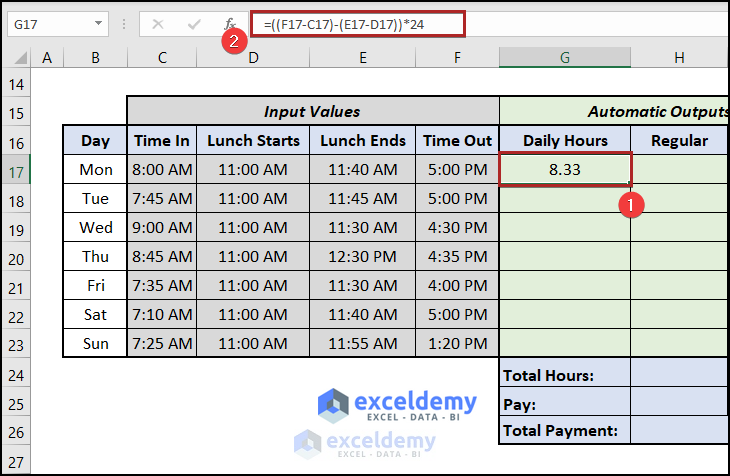
- In cell G17, enter the following formula:
=((F17-C17)-(E17-D17))*24
The C17 and F17 cells represent the Time In and Time Out while the D17 and E17 cells refer to the Lunch Starts and Lunch Ends times respectively. (F17-C17) is actually (Time Out – Time In), and (E17–D17) is (Lunch Ends – Lunch Starts). We multiplied ((Time Out – Time In) – (Lunch Ends – Lunch Starts)) by 24 to convert it into an hour value. This returns the value in Number format. Otherwise, subtraction of two times results in Time format.
- Press the ENTER key.
- Bring the cursor to the bottom right corner of cell G17 to activate the Fill Handle tool.
- Double-click on it to Autofill the other cells in the range.
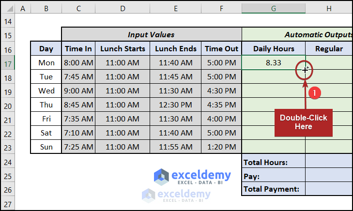
The formula is copied to the remaining cells in the G18:G23 range.
Step 5 – Determine Overtime
Before calculating Regular Hours, we calculate the Overtime Hours using the IF function.
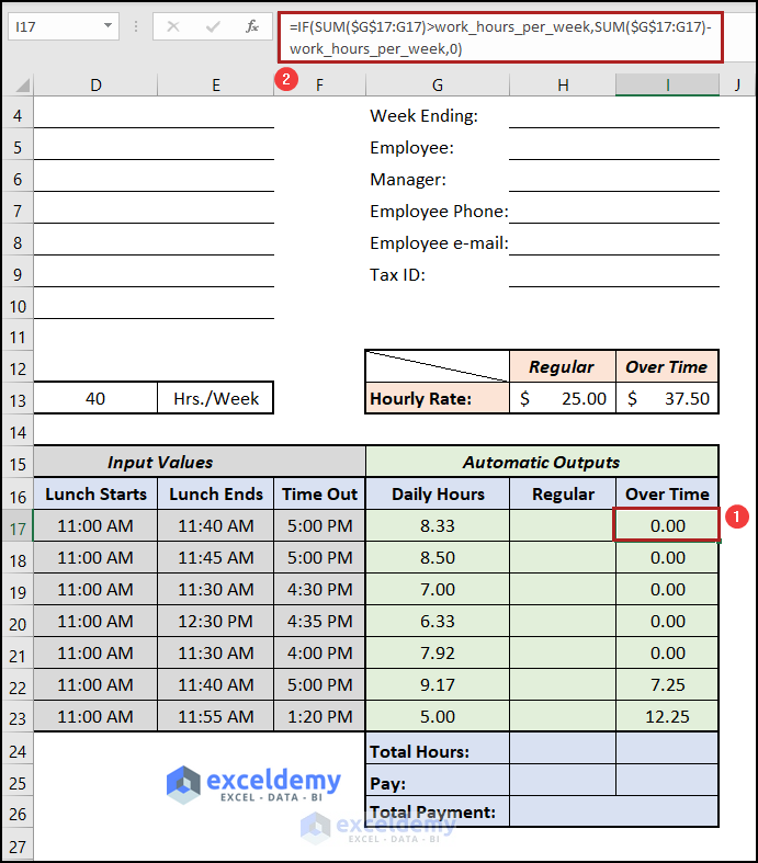
- In cell I17 enter the following formula:
=IF(SUM($G$17:G17)>work_hours_per_week,SUM($G$17:G17)-work_hours_per_week,0)
where work_hours_per_week represents cell D13.
- This formula has an expanding range. For cell I17 it is $G$17:G17. For the next cell (I18) in the column, the range will expand to $G$17:G18.
- logical_test: Checks whether the sum of the expanding range has exceeded the value of work_hours_per_week.
- value_if_true: If the sum exceeds the value, the value returned is: SUM($G$17:G17)-work_hours_per_week.
- value_if_false: Otherwise, the IF function returns a value of 0.
- Press ENTER.
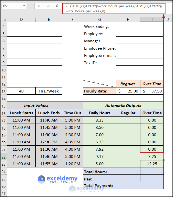
To check this formula in cell I22, enter:
=IF(SUM($G$17:G22)>work_hours_per_week,SUM($G$17:G22)-work_hours_per_week,0)
=IF(47.25>40,47.25-40,0) [some parts of the formula have been replaced with their values]
=IF(TRUE,7.25,0)
=7.25
So, the formula returns a value of 7.25.
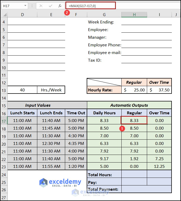
Step 6 – Compute Regular Time
Now we’ll use the MAX function to compute Regular Time.
- In cell H17 enter the formula below:
=MAX(G17-I17,0)
This formula returns the maximum of the two values G17-I17 and 0.
- Press ENTER.
Step 7 – Enumerate Total Weekly Hours
With all the base data input, we can now calculate the Total Regular Hours and Total Over Time Hours.
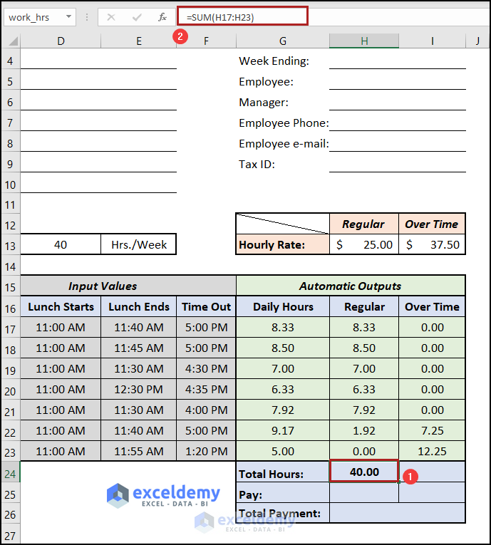
- In cell H24 enter the following formula:
=SUM(H17:H23)
17:H23 represent the cells containing Regular Hours in a week. We used the SUM function to sum up the values in these cells.
- Press ENTER.
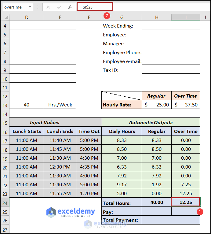
- In cell I24 enter the following formula:
=$I$23
Cell I23 holds our Total Overtime hours, because it represents the cumulative overtime for the week.
- Press ENTER.
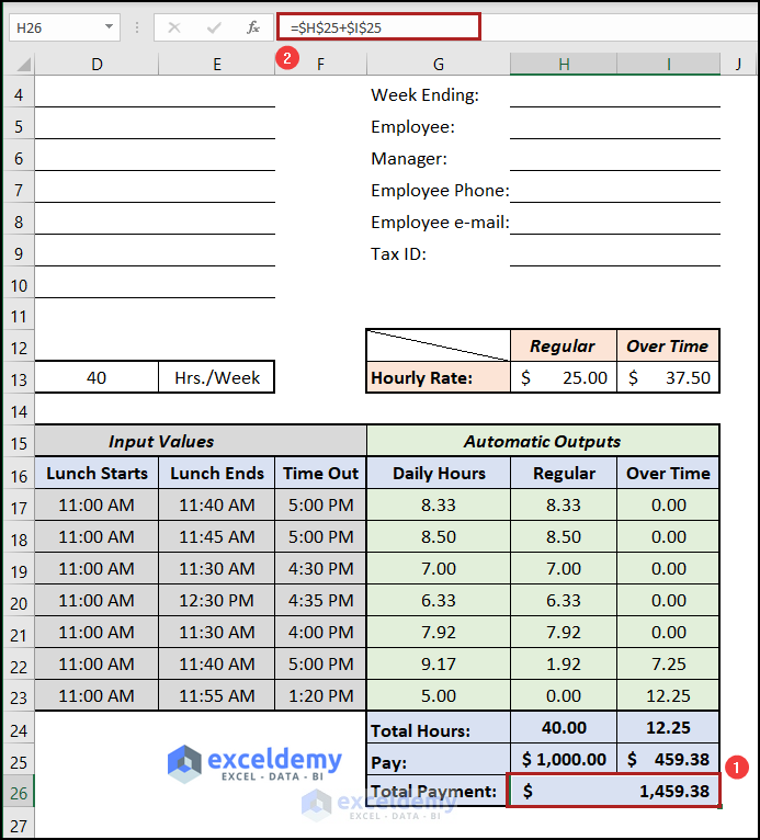
Step 8 – Estimate Total Payment
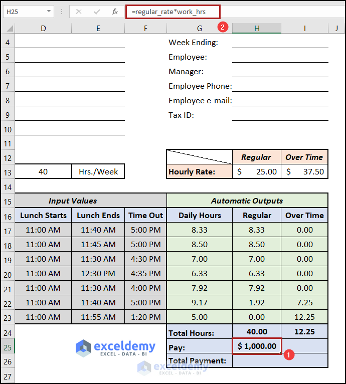
In cell H25, we calculate the Total Regular payment due. The formula is the following:
=regular_rate*work_hrs
This is simply the multiplication of the Regular Hourly Rate by total Regular Hours.
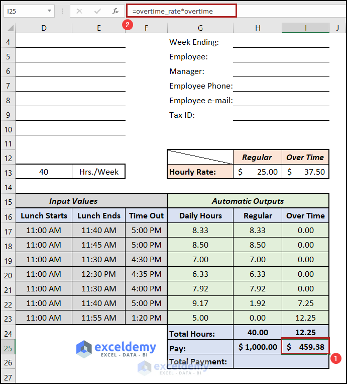
And we calculate the total Overtime Pay in cell I25. The formula for this is as follows:
=overtime_rate*overtime
This is simply the multiplication of Over Time Rate by Over Time Hours.
Now we can calculate the Grand Total Payment by adding up both the previously calculated payment types.
- In cell H26, enter the following formula:
=$H$25+$I$25
Bonus Template
This Excel template below can be used directly in your workplace, and will print out on one page (in Letter and A4 format with Landscape orientation) without any modification.
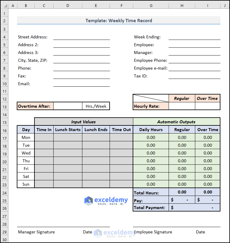
Necessary Inputs:
Put the following inputs in the Excel template:
Overtime After: Enter 40 for 40 hours per week. If your office maintains different working hours, input that value instead.
Hourly Rate: Regular Hourly Rate is usually less than the Overtime Hourly Rate.
Regular: Input the regular hourly rate.
Over Time: Input the overtime hourly rate.
The template takes 4 different time inputs (see the above image):
Time In: The time when the employee enters the working place.
Lunch Starts: The time when lunch starts in the working place.
Lunch Ends: The time when the employee ends lunch.
Time Out: The time when the employee leaves the office.
How to Calculate Overtime for Monthly Salary Employees?
In the previous steps, we used the example of an employee who is paid on a weekly basis. Below is a timesheet for employees who receive salaries on a monthly basis.
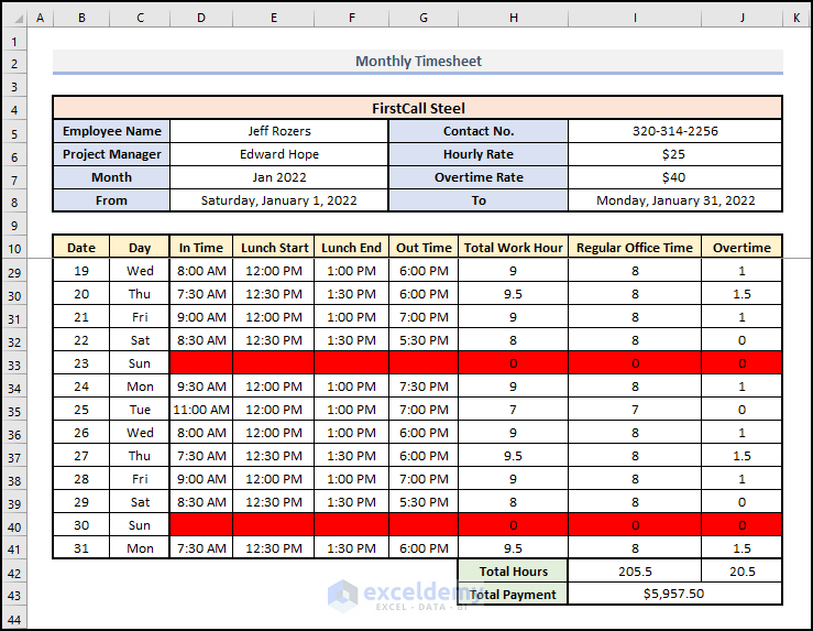
Here, we assumed a weekly holiday of one day.
<< Go Back to Overtime | Formula List | Learn Excel
Get FREE Advanced Excel Exercises with Solutions!

Good. Send me learning module of Excel in my e-mail I’d: [email protected]
Thanks, Ghosh for your feedback.
What if your company rounds the time? For example: When I clock in at 06:07 it calculates my time starting at 06:00 but if I were to clock in at 06:08, my start time is calculated at 06:15. By the way, Your emails are great. I highly enjoy them.
Hi BRIAN WINKLE,
Sorry for the late reply. I am replying to you on behalf of Exceldemy. To create a timestamp like the given example, you can take a look at the article below.
https://www.exceldemy.com/create-a-timesheet-in-excel/
I hope this will help you to solve your problem.
Thanks!
I will check this issue and let you know. Glad to know that we can add some value via our emails.
Best regards
Kawser
These formulas work pretty good if you work the 1st or 2nd shift. I work from 11:00pm – 7:30am with a 1/2 lunch period. When I enter these times, the formulas do not work. Any way to update this to work with these start and stop times?
Hi JIM,
Sorry for the late reply. I am replying to you on behalf of Exceldemy. You need to apply the formula below in Cell G16:
=24-((C16-F16)-(D16-E16))*24I hope this will help you to solve your problem. Please let us know if you have other queries.
Thanks!
Hi sir
Please send me practice data for advanced Excel so I can practice.
Thanks
Mdu
You will also find the file in our article. The file is at the upper part of the article. You will find the file under this title: “Calculate Hours Worked and Overtime Excel Template”.
Best regards
Kawser Ahmed
In the overtime column, it is calculating the total overtime for the week. What if you wanted to just calculate the overtime hours for that day. For example in cell I22, instead of reading the total for the week (12.25) it just read the overtime for that day (5.0).
Thank You!!
Hi JOE FRAZIER,
Thanks for your comment. I am replying to you on behalf of Exceldemy. In this article, Cells I16:I22 of Column I counts the overtime for each day of a week. That means if you want to see the overtime for Monday, you need to check Cell I16. So, you can use the same formula to calculate overtime for a single day.
I hope this will help you to solve your problem. Please let us know if you have other queries.
Thanks!
This was exactly what I was looking for! Is there a way for it to be multiple employees, in a table format verse just an individual log? Playing around with the formula now, seeing how I can enter more than one employee and the formula continues correctly
Thanks, Christina for your feedback. Glad to know that it helped you someway.
Kawser,
Please help me…I’m stuck on step 2. The overtime formula refers to “work_hours_per_week”, but I don’t see that specific name anywhere on the spreadsheet. Is that written somewhere for it to pull from? I’m trying to create a spreadsheet of my own following the format, but how can I get it to pull from a cell without a name?
Hi DEE ZELAYA,
Sorry for the late reply. I am replying to you on behalf of Exceldemy. Here, Cell D12 is renamed as work_hours_per_week. You can use the Name Manager in the Formulas tab to define the name. To check the defined names, follow the steps below.
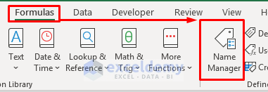
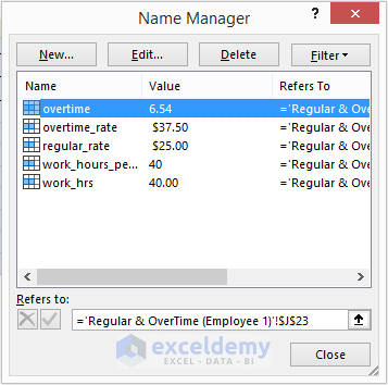
Firstly, download the practice book, go to the Formulas tab and select Name Manager.
In the Name Manager box, you will find all the defined names.
To apply the same formula in your new spreadsheet, you need to define the names using the Name Manager. To do that, you can follow the link below.
https://www.exceldemy.com/excel-edit-named-range/
Thanks!
Maybe a bit late for a reply, but I only came across this today.
The cell where it says 40, is renamed as work_hours_per_week
Top left next to the function bar you can rename a cell you choose
Please help me…I’m stuck on step 2. Name appears in the Colum or sum
Hi FEITY LAU,
Sorry for the late reply. I am replying to you on behalf of Exceldemy. I guess you are facing the problem because of not defining the names. Here, Cell D12 is renamed as work_hours_per_week. You can use the Name Manager in the Formulas tab to define the name. To check the defined names, follow the steps below.


Firstly, download the practice book, go to the Formulas tab and select Name Manager.
In the Name Manager box, you will find all the defined names.
To apply the same formula in your new spreadsheet, you need to define the names using the Name Manager. To do that, you can follow the link below.
https://www.exceldemy.com/excel-edit-named-range/
Thanks!
When I do this my mins are always off. example:
Shift start (E6)
0756
lunch start (F6)
1325
lunch end (G6)
1354
shift end (H6)
1635
My read back is 8 hr and 17 min. However, it should be 8 hr and 10 min.
I used the above formula:
=((H6-E6)-(G6-F6))*24
Am I missing something?
Also, the return time for G16 above appears to me to be wrong. After I converted it to military time the return time should have been 8.20 or 8 hours and 20 min. and shown is 8.33 or 8 hrs and 33 min.
Hi CHRISTIAN,
Thanks for your comment. I am replying to you on behalf of Exceldemy. The time difference in the above article is in Number format. That is why 8.17 doesn’t mean 8 hours 17 min. It actually means 8 hours and 10 minutes. To get the results in the desired format, you can follow the steps below.
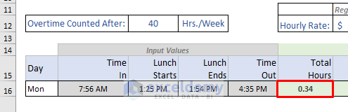
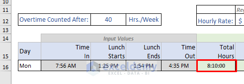
First of all, select Cell G16 in the dataset and type the formula below:
=((F16-C16)-(E16-D16))Hit Enter to see the result.
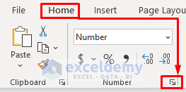
Select Cell G16 again, go to the Home tab, and click on the Number Format icon. It will open the Format Cells window.
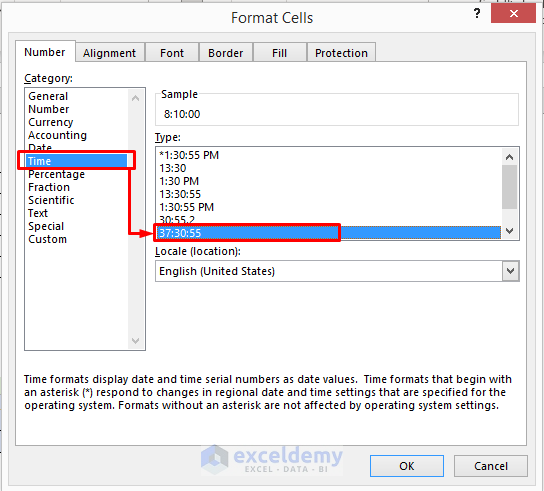
In the Format Cells window, click on the Number tab and select Time.
Then, select 37:30:55 from the Type box.
As a result, you will see the result in the desired format.
I hope this will solve your problem. Please let us know if you have any other queries.
Thanks!
I have created a time sheet to track my own hours and pay for years now. However the new job I have started I am changing to overnights and this formula and sheet is showing negative hours instead of positive. How can this be fixed? Been trying to figure out the formula to calculate overtime over 40 hours and cannot seem to figure this one out – HELP lol…
Hi JASON,
Thanks for reading our articles. You have mentioned that you are getting negative hours due to overnight. You can solve this easily. Insert the following formula on cell G17:
=24-((C17-F17)-(D17-E17))*24
Hope, this will help you to solve your problem. Please let us know if you have other queries.
Thanks!
Alok, ExcelDemy