Here’s the dataset we’ll use to count rows.
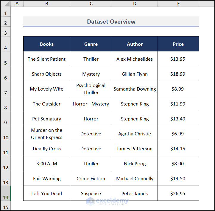
We have a table with three columns; Books, Genre, and Author. There are 10 books listed. To show the count of visible rows, we will apply filters on the table. This will hide a few rows and you can understand the differences.
For counting rows, you can use the COUNTA function in the result cell:
=COUNTA(E5:E14)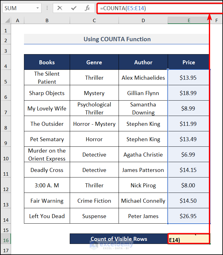
- Press ENTER and you will get the result like the image below.
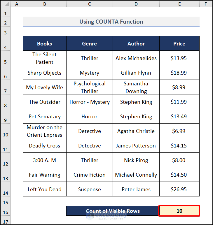
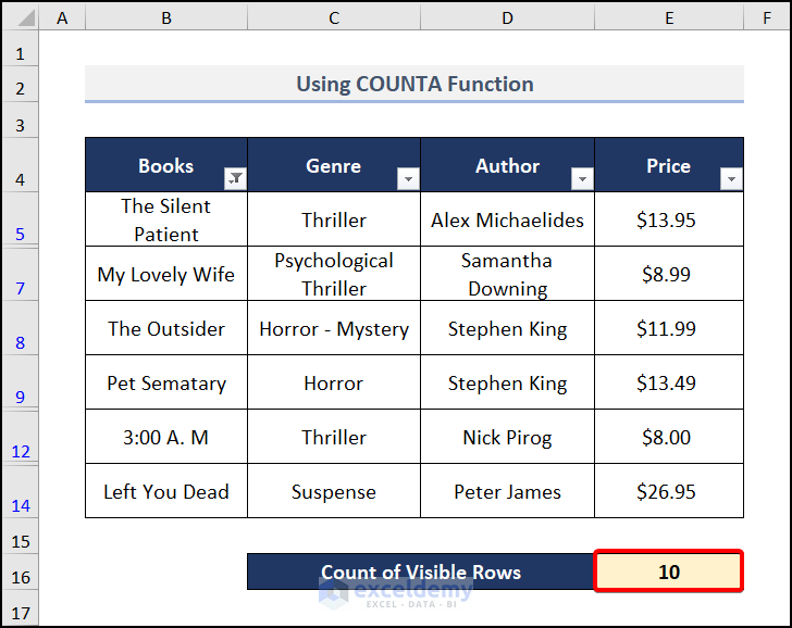
- If you filter your data, this function will still count the hidden rows.
Method 1 – Using the SUBTOTAL Function
The SUBTOTAL function takes a func_num to do the specific operation and a data range to apply it on. As we want to count the visible rows, we will use the COUNT and COUNTA functions. For text values, we need to use the COUNTA function. So our function_number should be 3. Follow the steps to do it.
Counting Visible Rows of Texts:
- Input the below formula in cell C17.
=SUBTOTAL(3,B5:B14)It checks for the B5:B14 cell and counts for the rows as we enter the func_num as 3 for the COUNTA function.
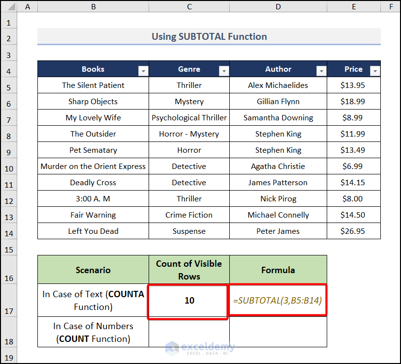
- We are showing examples using the Books column within our range. You can choose any of the columns. It gave the rows that are visible.
- Use a filter (this will make some rows visible and some invisible).
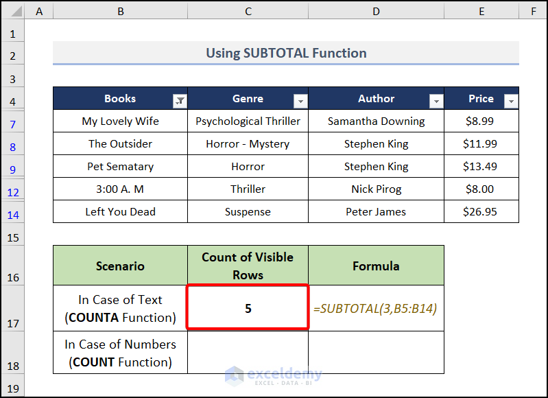
We have filtered by Books and 5 rows are visible. Our formula returned the correct result.
You can also use the COUNT function instead of the COUNTA function in the case of text values. Here the function number is 2.
Counting Visible Rows of Numbers:
- Go to cell C18 and insert this formula:
=SUBTOTAL(2,E5:E14)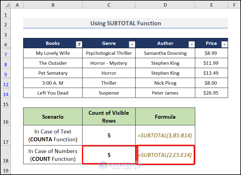
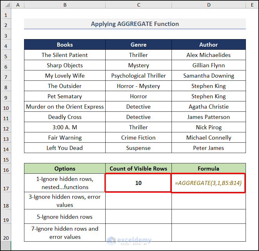
Method 2 – Utilizing the AGGREGATE Function
The AGGREGATE function does several tasks, so the number of functions is predefined within it.
Case 1
- Move to cell C17 and enter this formula.
=AGGREGATE(3,1,B5:B14)The second argument 1 ignores hidden rows and other aggregate functions. We put 3 in the function_number to use the count function.
Case 2
3 in the behavior_option argument ignores hidden rows and error values.
- Go to cell C18 and insert the formula.
=AGGREGATE(3,3,B5:B14)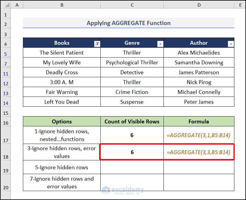
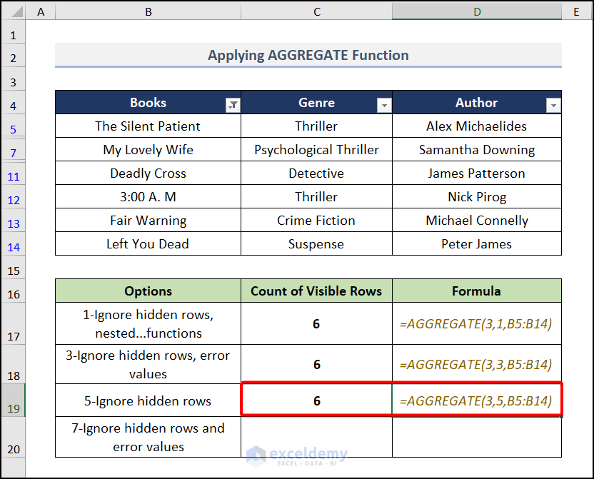
Case 3
We’ll use 5 in the behavior_option argument which is ignoring hidden rows.
- Go to cell C19 and use this formula:
=AGGREGATE(3,5,B5:B14)Earlier options (1 and 3) did the same, but that will take more time since their mechanism is such that they will also evaluate SUBTOTAL – AGGREGATE or error values.
Case 4
We’ll use 7 in the behavior_option argument which is for ignoring hidden rows and error values.
- Apply the below formula in cell C20:
=AGGREGATE(3,7, B5:B14)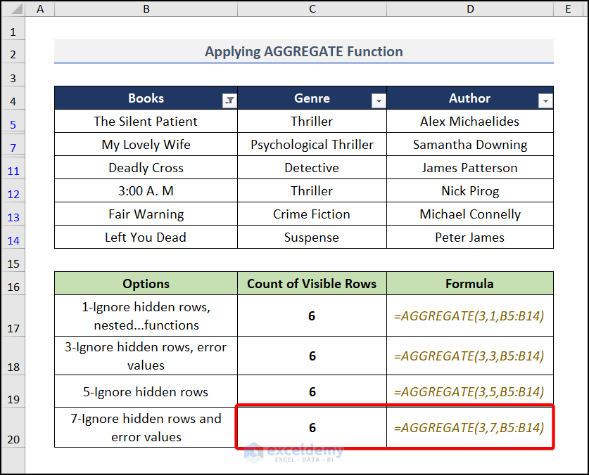
Method 3 – Applying VBA Code
Steps:
- Go to the Developer tab and choose Visual Basic.
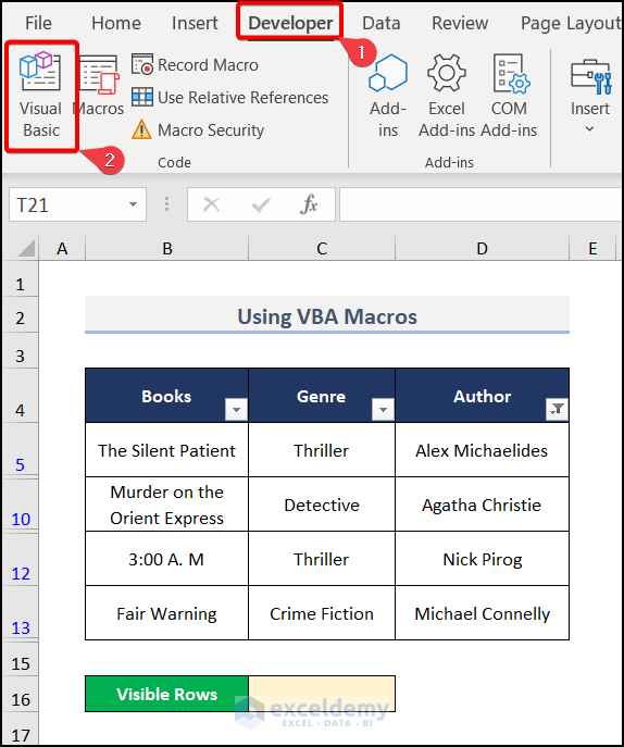
- A window will appear. Select Insert, choose Module, and pick Module1.
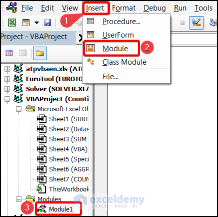
- Insert the VBA code in the General box.
Function COUNTVISIBLE(range)
Dim xCount As Long
Dim xCell As range
Application.Volatile
For Each xCell In range
     If (Not xCell.EntireRow.Hidden) And (Not xCell.EntireColumn.Hidden) Then
          xCount = xCount + 1
     End If
Next
    COUNTVISIBLE = xCount
End Function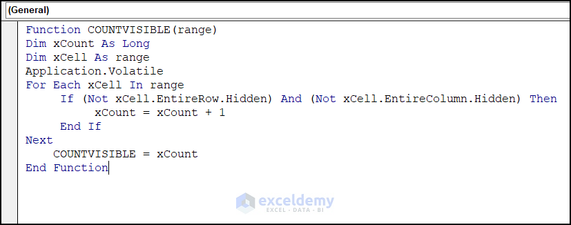
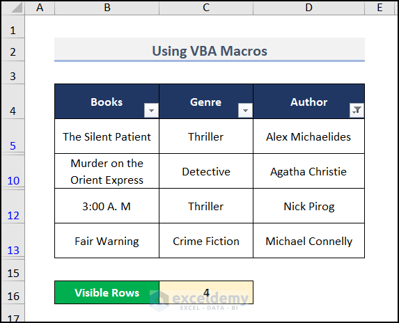
- Put the following formula with the created COUNTVISIBLE function in the C16 cell.
=@COUNTVISIBLE(C5:C14)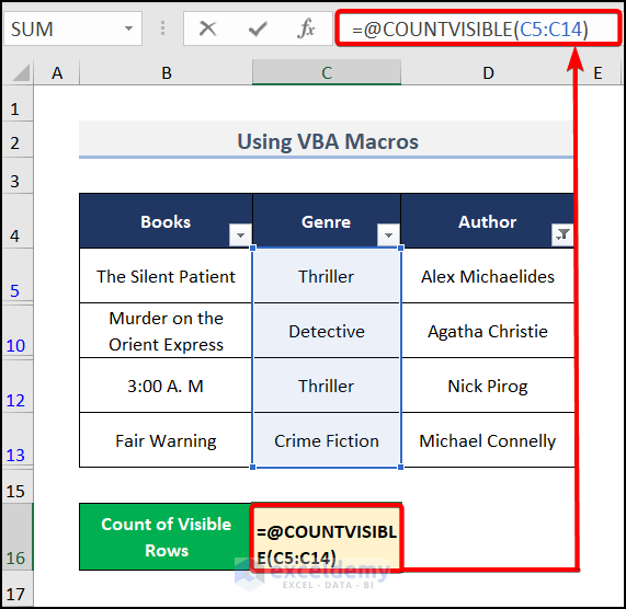
You will get the desired result.
How to Count Visible Rows with Criteria
Example 1 – Criteria with OFFSET Function
Steps:
- Move to cell C19 and insert the following formula:
=SUMPRODUCT(SUBTOTAL(3, OFFSET(C5:C14, ROW(C5:C14)-MIN(ROW(C5:C14)),,1)), --(C5:C14=C16))C5:C14= The text value of “Genre”.
C16= The Seach Key “Detective” in C16.
Formula Explanation:
In the above formula, we checked the key value within the range and it returns an array of TRUE and FALSE. The double unary operator (—) converts the TRUE and FALSE values into 1s and 0s.
The subtraction of 2 ROW functions provides an array of rows, starting from 0. This array will work as rows inside the OFFSET function.
We are setting a range, an array of rows, and 1 as height inside the OFFSET function. This will provide an array of entire values within the range.
The SUBTOTAL function converts the array returned by the OFFSET function into an array of 1’s and 0’s where 1’s represent visible cells and 0s match hidden cells.
The SUMPRODUCT function has two arrays of 1’s and 0’s. It multiplies the arrays and then calculates the sum.
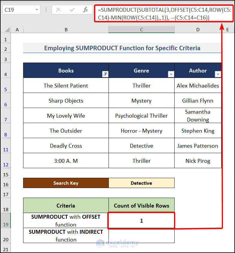
You will get the result like in the above image. It counts the rows for our searching text “Detective”.
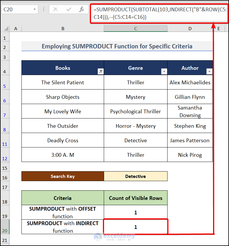
Example 2 – Criteria with INDIRECT Function
Steps:
- Go to cell C20 and insert this formula.
=SUMPRODUCT(SUBTOTAL(103, INDIRECT("B"&ROW(C5:C14))),--(C5:C14=C16))Formula Explanation:
We checked the key value within the range and it returns an array of TRUE and FALSE. The double unary operator (–) converts the TRUE and FALSE values into 1’s and 0’s.
We have a ROW function inside the INDIRECT function. We need to set a column name within the INDIRECT function.
We have written “B” inside the ROW function given the range B4:B13. This will give an array of entire values within these cells.
The SUBTOTAL function converts the array returned by the INDIRECT function into an array of 1’s and 0’s where 1s represent visible cells and 0s match hidden cells.
The SUMPRODUCT function has two arrays of 1s and 0s. It multiplies the arrays and then calculates the sum.
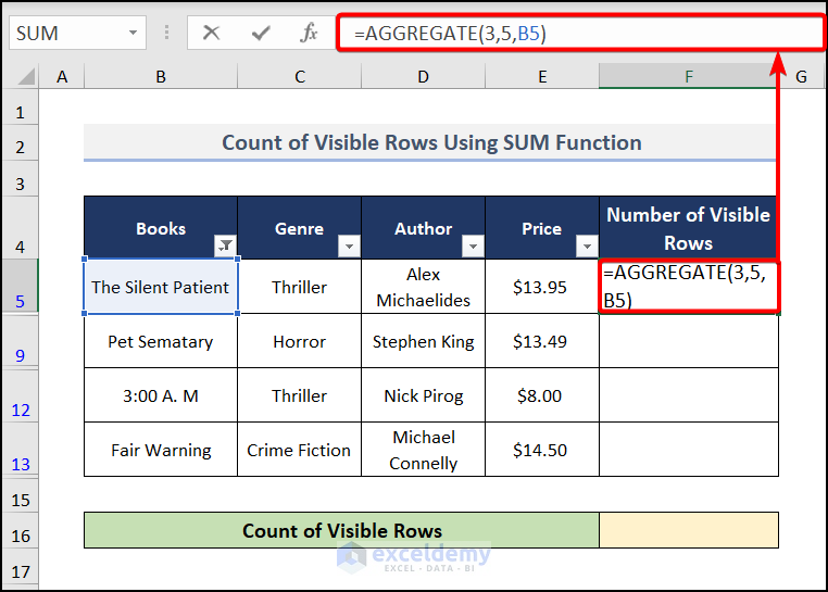
How to Count Visible Rows in a Filtered List
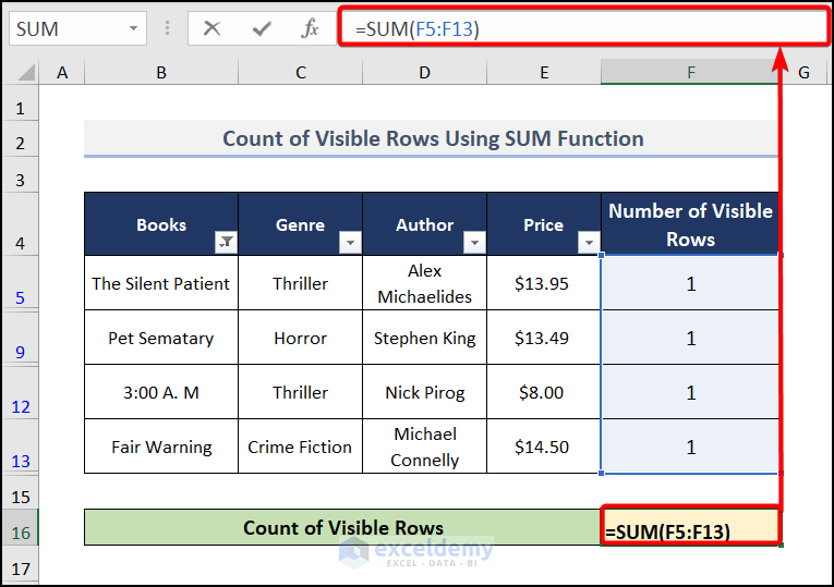
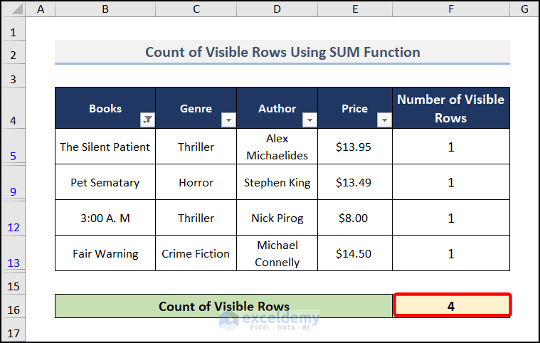
- Go to cell F5 and enter this formula.
=AGGREGATE(3,5,B5)In the AGGREGATE function, the first number (3) represents the function type (in this case, COUNTA to count non-empty cells), and the second number (5) is an option to ignore hidden rows and errors. This formula counts non-empty cells in B5, ignoring hidden rows and errors.
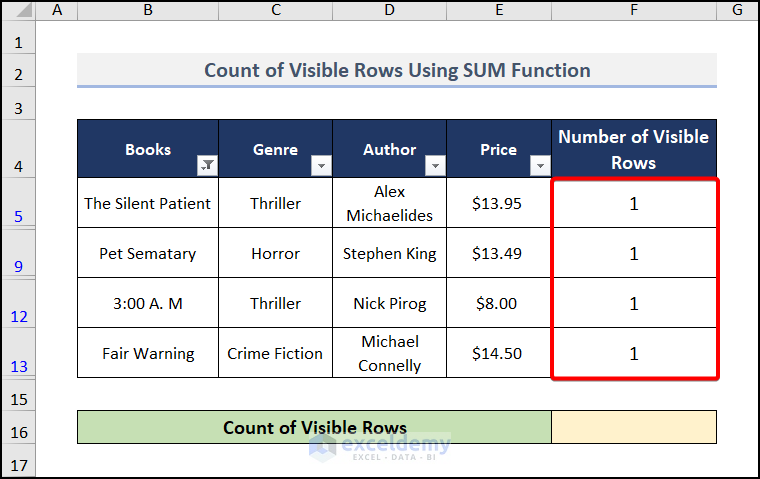
- Press Enter and drag down for other visible rows to find the output just like in the image below.
- Move to cell F16 and insert the formula.
=SUM(F5:F13)This SUM(F5:F13) syntax calculates the value from F5:F13 cells, which is the visible rows in our worksheet.
- You will get the result after pressing ENTER.
Practice Section
We have provided a practice section on each sheet on the right side so you can test these formulas.

Download the Practice Workbook
<< Go Back to Count Rows | Formula List | Learn Excel
Get FREE Advanced Excel Exercises with Solutions!

You don’t explain in the last example what the 3 & 5 represent in the formula =AGGREGATE(3,5,B5) ?
Thanks
Hello Rose Marra,
The formula =AGGREGATE(3,5,B9) uses the AGGREGATE function, which can perform various operations on a range, such as summing, averaging, or finding the largest value, while ignoring errors or hidden rows.
Here’s a breakdown:

3: This is the function number, specifying that the formula will perform the COUNTA function, which counts non-empty cells.
5: This is the options argument, where 5 means the function will ignore hidden rows and error values (e.g., cells with errors or those hidden by filters).

So, this formula counts the non-empty cells while ignoring any hidden rows and errors.
Regards
ExcelDemy