How to Count Filtered Rows with Criteria in Excel (5 Easy Ways)

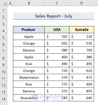
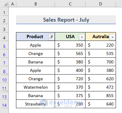
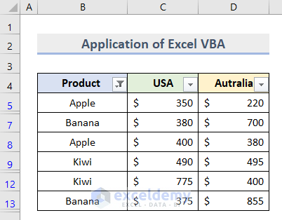
For illustration, here is a dataset with the July Sales Report of fruit sales in the USA and Australia.

Filter this dataset.

• Select cell range B4:D14.
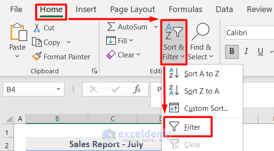
• Go to the Home tab and select Filter from the Sort & Filter drop-down in the Editing group.

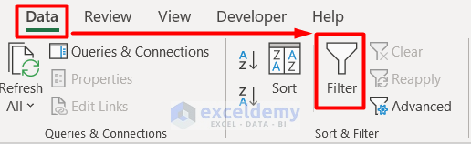
• The Filter tool in the Sort & Filter group can also be found under the Data tab.

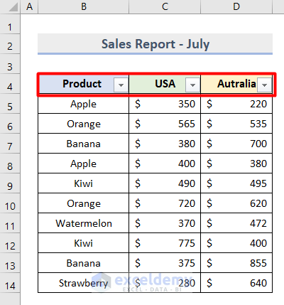
• The filter will be enabled in the dataset.

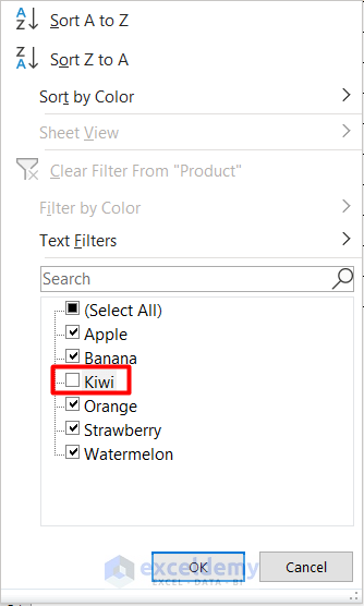
• To filter this, click on the arrow beside the Product column.
• We deselected Kiwi as we wanted to filter the other values.
• Click OK.

• You will get your filtered rows without the row for Kiwi.

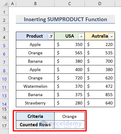
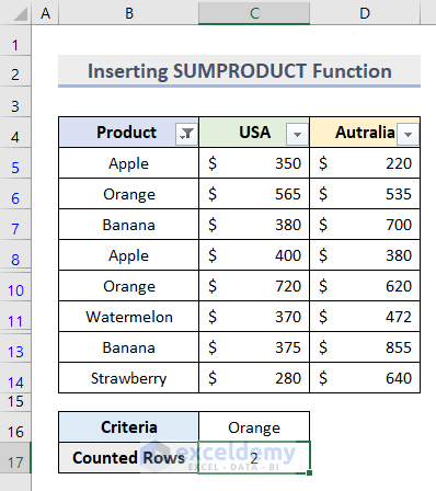
Method 1 – Insert SUMPRODUCT Function to Count Filtered Rows with Criteria in Excel

• Insert your preferred criteria for which you want to count rows.
• We gave the product Orange as the Criteria in cell C16.

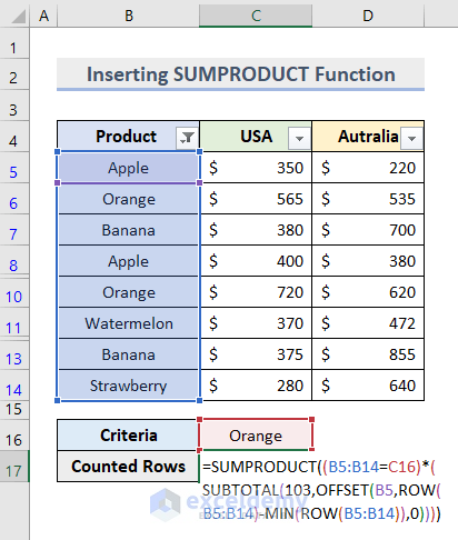
• Insert this formula in cell C17.

• Press Enter.
• It will display the number of rows containing the special criteria.

Method 2 – Count Filtered Rows with Criteria Using SUBTOTAL Function

• Insert this formula in cell C16.

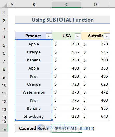
• Press Enter.
• We have created the general formula which will be applicable to any number of rows.
• It shows the total number of rows before filtering.

We used the SUBTOTAL function to return the total number of selected criteria. The function_num argument is defined as 3 to specify the COUNTA function for visible cells in the cell range B5:B14.

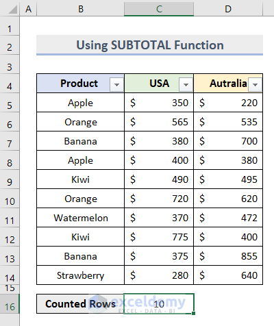
• Specify the criteria from the Filter context menu. We deselected Kiwi, Strawberry, and Watermelon.

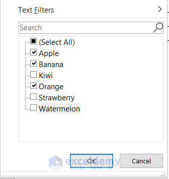
• Press OK.
• The filtered rows with criteria will be counted and the result will be displayed in cell C16.

Read More: How to Count Visible Rows in Excel

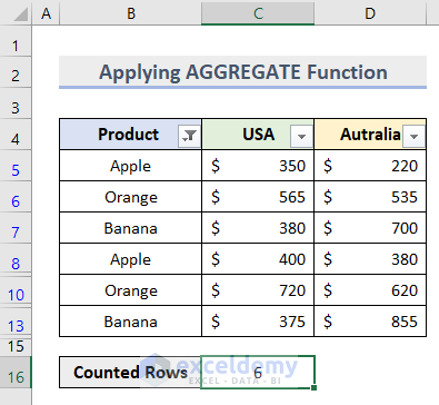
Method 3 – Apply AGGREGATE Function for Counting Filtered Rows with Criteria in Excel

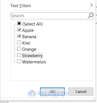
• Filter the product names Apple and Banana defining them as criteria.

• Insert this formula in cell C16.

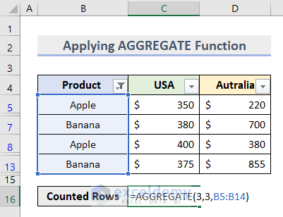
• Press Enter.
• It will show the number of rows for the selected criteria.

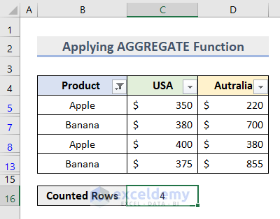
The AGGREGATE function creates the opportunity to avoid hidden rows or error values from the cell range B5:B14.

• To verify the formula, add Orange to the criteria from the Filter list.

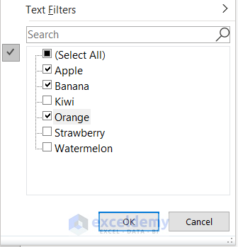
• Click OK.
• The number for counted rows will change.

Method 4 – Count Filtered Rows with Criteria Inserting Help Column

• Create a Help Column beside the original filtered dataset.
• Insert this formula in cell D5.

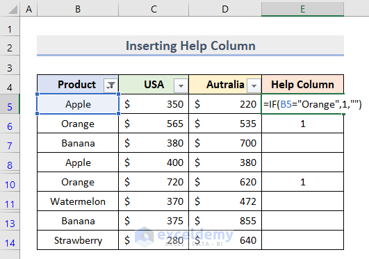
• Press Enter.
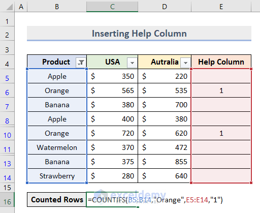
• Use the Fill Handle tool to drag this formula up to cell E14.

W used the IF function to compare our selected criteria Orange with the value in cell B5.

• Insert this formula in cell C16.

• Press Enter and it will output the counted value of filtered rows with criteria.

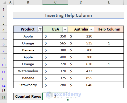
We applied the COUNTIF function to count cell range B5:B14 which meets the condition in cell range E5:E14.

Method 5 – Excel VBA to Count Filtered Rows with Criteria

• Filter your dataset according to your preferred criteria.

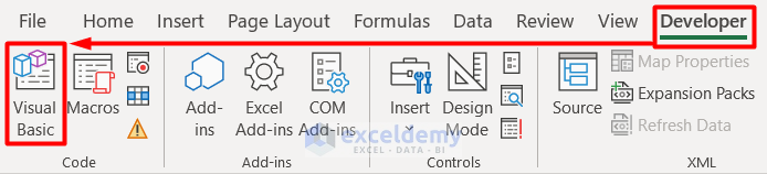
• Go to the Data tab and select Visual Basic under the Code group.

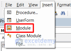
• Choose Module from the Insert section.

• Insert this code on the blank page.

Function COUNTVISIBLE(Rw)
    Dim xCnt As Long
    Dim xRng As Range
    Application.Volatile
    For Each xRng In Rw
        If (Not xRng.EntireRow.Hidden) And (Not xRng.EntireColumn.Hidden) Then
            xCnt = xCnt + 1
        End If
    Next
    COUNTVISIBLE = xCnt
End Function

• Save the code and close the window.
• Insert this formula in cell C16.

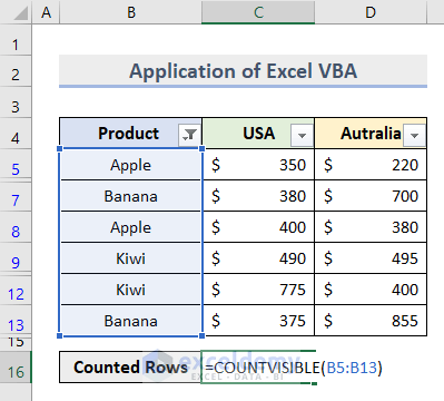
• Press Enter and it will show the number of visible rows.

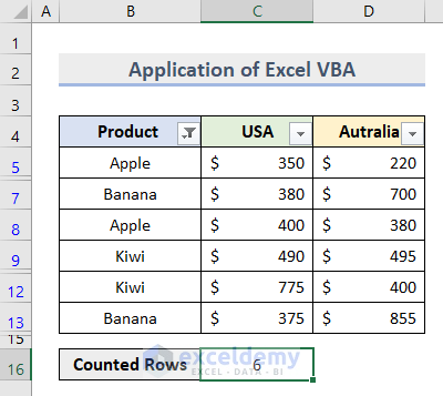
We applied the COUNTVISIBLE function to calculate the visible cells in the dataset. It will ignore the hidden cells during counting.

Download Practice Workbook

<< Go Back to Count Rows | Formula List | Learn Excel