How to Count Rows with Multiple Criteria in Excel (6 Methods)

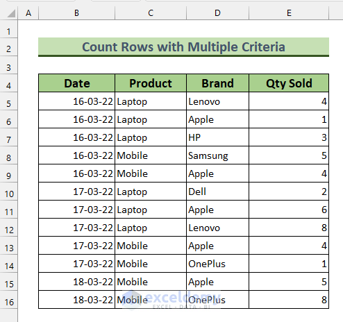
We have a dataset of a computer and mobile retailer showing daily product sales. It has four columns: date, Product, Brand, and Quantity Sold (Quantity). We will count rows that fulfill our given criteria.

Method 1 – Using the COUNTIF Function to Count Rows with Multiple Text Criteria in Excel

Steps:

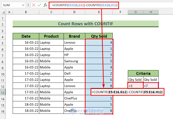
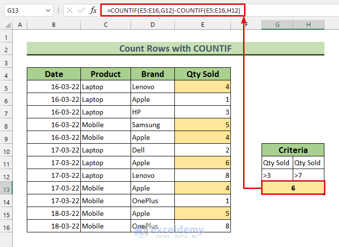
• Select an empty cell. Here, we selected cell G13.
• Enter the following formula:

We are using the COUNTIF function twice. The first time, it counts the values of Qty Sold that are more than 3 based on criteria greater than 3. The second time, it counts values based on criteria more than 7 of the Qty Sold column. Finally, it takes the difference to find our desired value.

• Press ENTER.

We will get the value 6. The values are highlighted in our rows to reflect our results.

Here, we use cell references in our formula. However, it can be done directly as well. To do it directly,

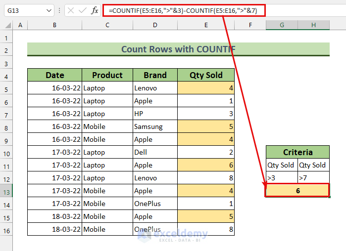
• Enter the following formula and then press ENTER:

We have counted rows that satisfy our criteria.

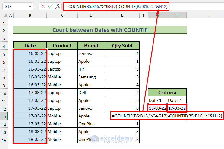
Method 2 – Applying the COUNTIF Function with Multiple Dates 

Steps:

• Enter the following formula in cell G13 (We’ve merged cell G13 and H13):

There are two COUNTIF functions in our formula. The first one counts the dates over 15 March and the second one counts the dates larger than 17 March. We are taking the difference between those two to find out our value.

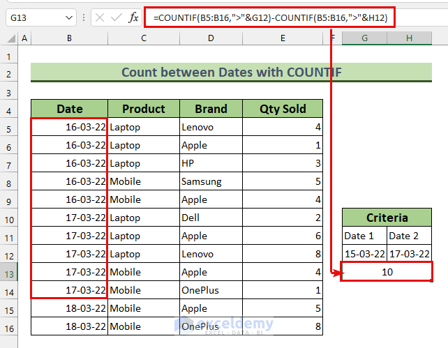
• Press ENTER.

Our count is 10 rows that fulfill our multiple criteria.

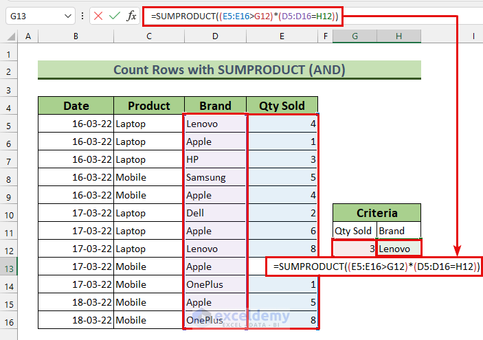
Method 3 – Using the SUMPRODUCT Function with AND Criteria to Count Rows in Excel

Steps:

• Enter the following formula in cell G13:

First, we find the Quantity(Qty) Sold more than 3. Then, we limit our findings to only the brand Lenovo. We use the multiple sign (*) for the AND operation.

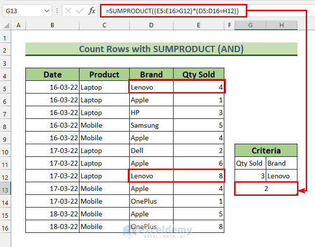
• Press ENTER.

We’ve found 2, which represents the number of rows maintaining the given criteria. If we check our dataset, there are two rows that have both “Lenovo” and “more than 3.”

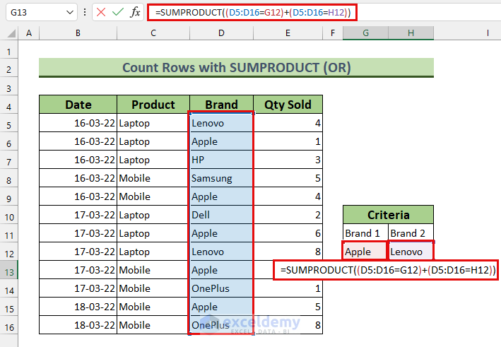
Method 4 – Counting Rows with Multiple Criteria in Excel Using the SUMPRODUCT Function with OR Criteria

Steps:

• Enter the following formula in cell G13:

We use the plus (+) sign for the OR operation. We get the number of rows with the text Apple or Lenovo.

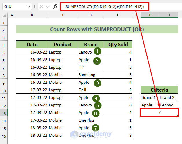
• Press ENTER.

The operation will show 7. We can see 7 instances of the two brands in our dataset.

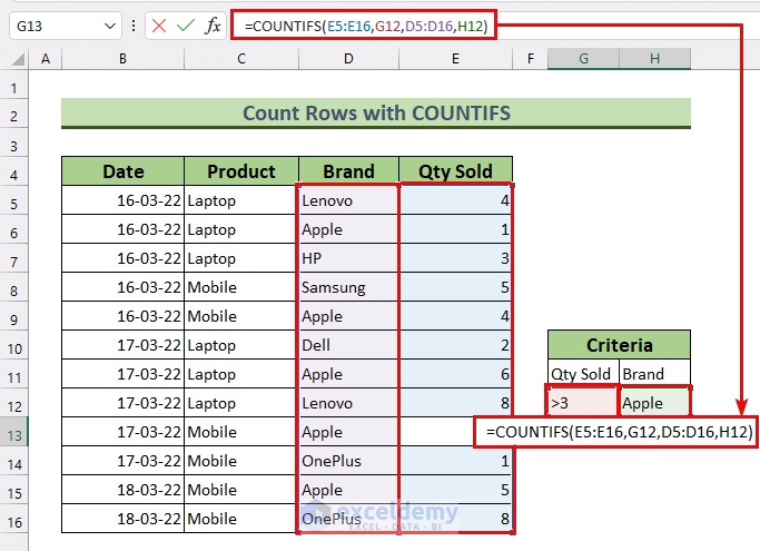
Method 5 – Utilizing the COUNTIFS Function Based on Multiple Criteria to Count Rows

Steps:

• Enter the formula below in cell G13:

Our formula sets the first criterion as Quantity(Qty) Sold more than 3 in cell G12, and Brand Apple in cell H12 as the second criterion.

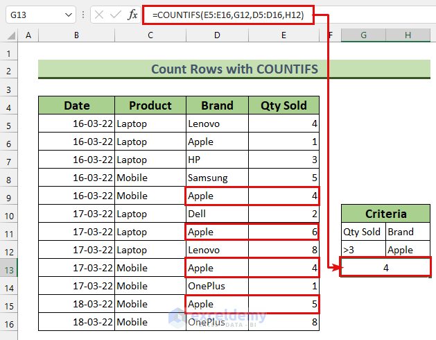
• Press ENTER.

The result is 4. We’ve marked our dataset to verify our formula. Our dataset shows four times when Apple products were sold in a quantity larger than 3.

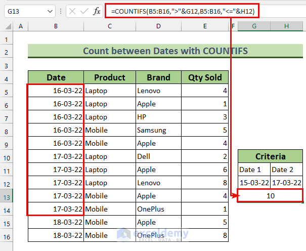
Method 6 – Employing the COUNTIFS Function with Multiple Dates as Criteria to Count Rows

Steps:

• Enter the following formula in cell G13:

The First part (B5:B16,”>”&G12) is to find the dates more than 15 March. And the next part (B5:B16,”<=”&H12) is finding the dates less or equal to 17 March.

• Press ENTER.

We will get our desired value. We count 10 rows that match our criteria.

Practice Section

In the Excel file, we have included practice datasets for every method to count rows with multiple criteria.

Download the Practice Workbook

<< Go Back to Count Rows | Formula List | Learn Excel