Problems with the Text and Number Formats in VLOOKUP
If your lookup value and the column values are in a different format, it will cause an error.
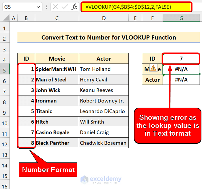
Consider this dataset.
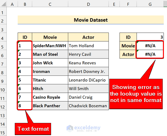
We used the following VLOOKUP formula to find the Movie name:
=VLOOKUP(G4,$B$4:$D$12,2,FALSE)
To get the Actor name, we used:
=VLOOKUP(G4,$B$4:$D$12,3,FALSE)
Our lookup value was in the number format and our lookup column has the text format. That’s why it couldn’t give us the result we wanted. We have to convert the number to get the actual result.
How to Convert Number to Text for VLOOKUP in Excel: 2 Ways
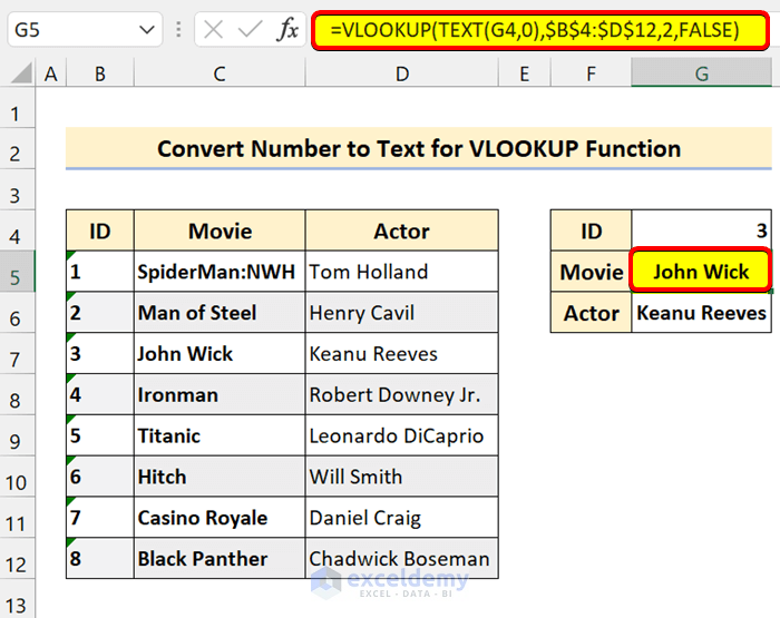
Method 1 – Use the TEXT Function to Convert a Number to Text for VLOOKUP
The Generic Formula:
=VLOOKUP(TEXT(cell,0),table_array,column_index_number,FALSE)
- To get the Movie name, use:
=VLOOKUP(TEXT(G4,0),$B$4:$D$12,2,FALSE)
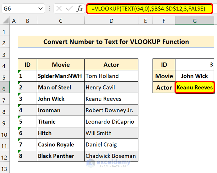
- To get the Actor name, use the following formula:
=VLOOKUP(TEXT(G4,0),$B$4:$D$12,3,FALSE)
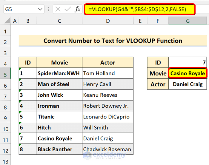
Method 2 – Concatenate with an Empty String to Convert a Number to Text
The Generic Formula:
=VLOOKUP(lookup_value&””,table_array,column_index_number,FALSE)
By concatenating (ampersand symbol for string values) with a blank string (nothing in double quotes), we can convert the lookup value from a number to text.
- To get the Movie name:
=VLOOKUP(G4&"",$B$4:$D$12,2,FALSE)
- To get the Actor name, use the following formula:
=VLOOKUP(G4&"",$B$4:$D$12,3,FALSE)

Read More: How to Convert Number to Text in Excel with Apostrophe
Important Tip
If you are not sure whether the lookup value is in the numbers or text format, use the IFERROR function as in the following formula:
=IFERROR(VLOOKUP(G4,$B$4:$D$12,2,FALSE),VLOOKUP(G4&"",$B$4:$D$12,2,FALSE))
The formula will try the VLOOKUP formula assuming that the lookup value and the first column in the table array are in numbers. If it returns an error, then it will try the next VLOOKUP formula. The next VLOOKUP formula will convert the number to text. If this also fails, it will throw the #N/A error.
Convert Text to Number for the VLOOKUP Function in Excel
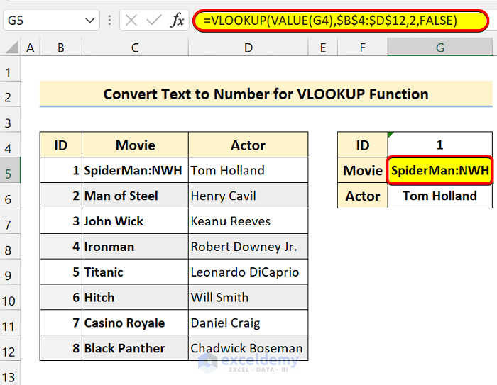
Consider the following dataset where the first column in the number format but the lookup value in the VLOOKUP function is in the text format.
You can use the VALUE function to convert text to numbers for the VLOOKUP formula in Excel.
The Generic Formula:
=VLOOKUP(VALUE(lookup_value),table_array,column_index_number,FALSE)
- To get the Movie name:
=VLOOKUP(VALUE(G4),$B$4:$D$12,2,FALSE)
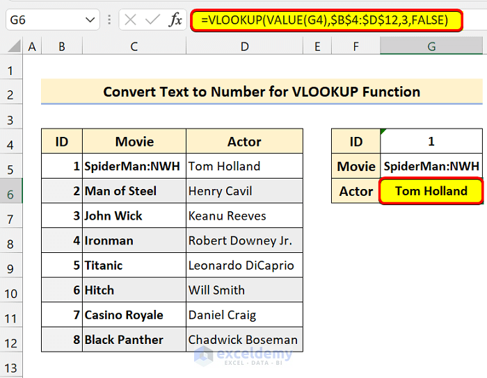
- Get the Actor name by using the following formula:
=VLOOKUP(VALUE(G4),$B$4:$D$12,3,FALSE)
Things to Remember
✎ If you are not sure about the formats, wrap the VLOOKUP in the IFERROR function as we discussed earlier.
✎ Turn on error checking to find the numbers stored as text.
Download the Practice Workbook
Related Articles
- Excel Convert Number to Text with Leading Zeros
- How to Convert Number to Text with Green Triangle in Excel
- How to Convert Number to Text and Keep Trailing Zeros in Excel
- Convert Number to Text without Scientific Notation in Excel
- How to Convert Number to Text with 2 Decimal Places in Excel
- Convert Number to Text with Commas in Excel
<< Go Back to Excel Convert Number to Text | Learn Excel
Get FREE Advanced Excel Exercises with Solutions!

HI, I HAVE A VLOOKUP FORMULA [=IF(ISNA(VLOOKUP((VALUE($A42)),PROJECT_LIST!$A:$C,3,FALSE)),””,VLOOKUP((VALUE($A42)),PROJECT_LIST!$A:$C,3,FALSE)&” “)] ITS WORKING WHEN IT LOOKUP ON NUMBERS BUT TO LOOKUP ON LETTERS WITH NUMBERS IT SHOWS ERROR (#VALUE).
Hello ARCHIE,
I understand you wish to fix the #VALUE! error for VLOOKUP. In your case, the reason this is returning #VALUE! error for alpha-numeric values is that it is trying to convert the text values to numbers using the VALUE function. The VALUE function is designed to convert text that represents a number to an actual number. When it encounters alpha-numeric values, it cannot convert them to numbers, hence the error.
Fortunately, you can fix this by modifying the formula by replacing the VALUE function with the TEXT function. The TEXT function converts a value to text in a specific number format. Try the modified formula given below:
=IF(ISNA(VLOOKUP(TEXT($A42,"0"),PROJECT_LIST!$A:$C,3,FALSE)),"",VLOOKUP(TEXT($A42,"0"),PROJECT_LIST!$A:$C,3,FALSE)&" ")Let me know with a demo dataset if you still face issues. Good luck!
Note: Make sure data are sorted in ascending to descending order in the lookup table.
Regards,
Yousuf Khan