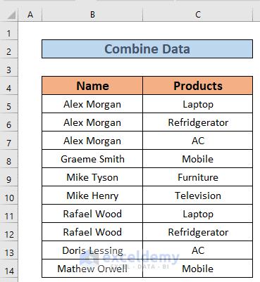
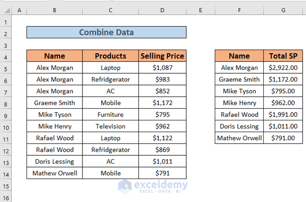
Here is the dataset we will use to explain the methods. We have some salespersons and a list of Products that they have sold. We will combine the same values.
How to Combine Cells with the Same Value in Excel: 3 Easy Ways
Method 1 – Using IF and CONCATENATE Functions in Excel to Combine Cells with the Same Value
Steps:
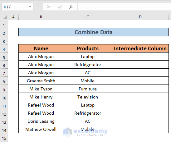
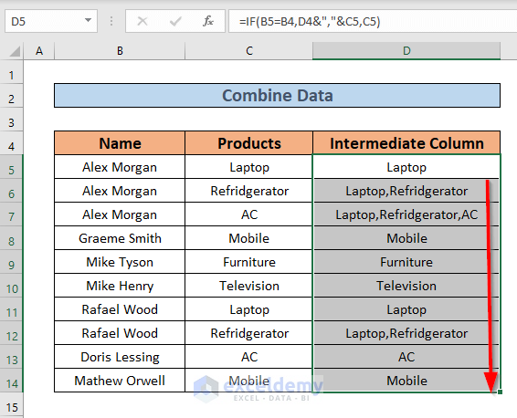
- Create an intermediate column D where all the items will be listed.
- Go to D5 and copy the following formula into it:
=IF(B5=B4,D4&","&C5,C5)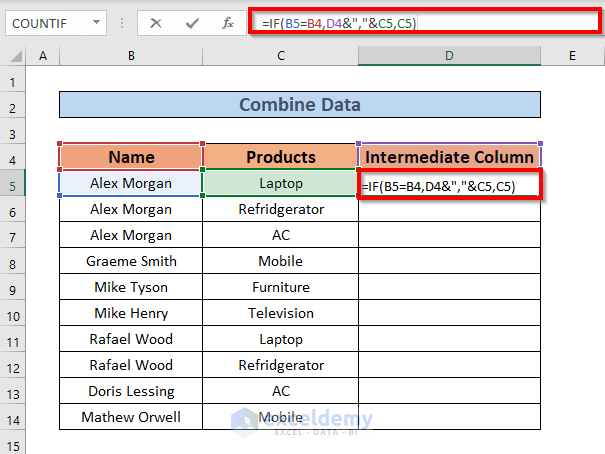
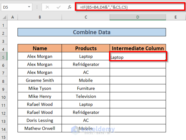
Here, in the IF function the logical statement is B5=B4. If this is TRUE, it will return D4&”,”&C5 (which eventually is Intermediate Column, Laptop), and if FALSE, it will give C5 as output. Since the statement is FALSE, we have C5 as output.
- Press Enter.
- Use the Fill Handle to AutoFill up to D14.
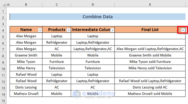
- Create a new column E for the “Final List”.
- Go to E5 and insert the following formula:
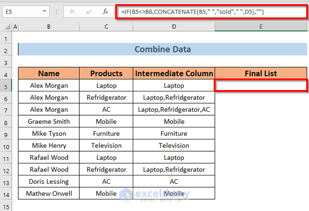
=IF(B5<>B6,CONCATENATE(B5," ","sold"," ",D5),"")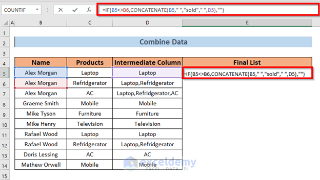
Formula Breakdown:
“ “ —> It creates space.
- CONCATENATE(B5,” “,”sold”,” “,D5) —> Concatenates the words or cells.
- Output: Alex Morgan sold Laptop
IF(B5<>B6,CONCATENATE(B5,” “,”sold”,” “,D5),””) —> Returns the output after analyzing the logical statement B5<>B6.
- IF(FALSE,{Alex Morgan sold Laptop},{})
- Output:{}
- Press Enter.
- Use the Fill Handle to AutoFill up to E14.

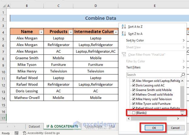
- Select the entire dataset.
- Go to the Data tab, select Sort & Filter, and choose Filter.
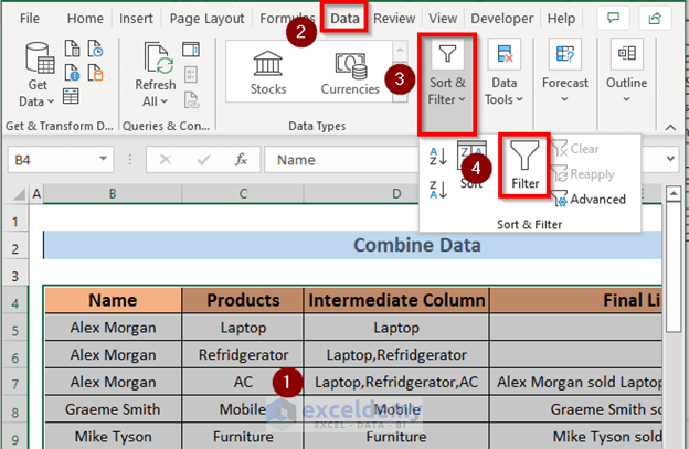
- Then select the drop-down (see image).
- Uncheck the Blanks option and click OK.
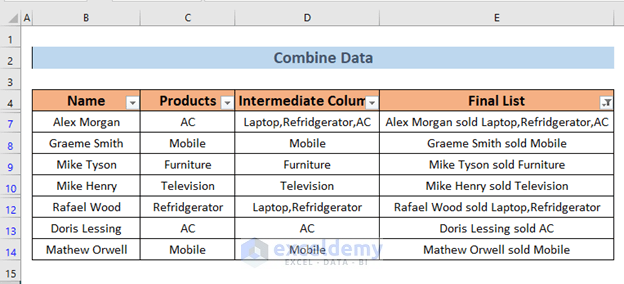
- You will get the list with the same values.
NOTE:
In this method, the same values should be next to each other. We have sorted the dataset in a way that the cells having Alex Morgan are adjacent to each other.
Read More: How to Concatenate Multiple Cells in Excel
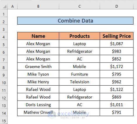
Method 2 – Using the Consolidate Feature to Combine Cells with the Same Value in Excel
We have added the Selling Price column to the dataset.
 Steps:
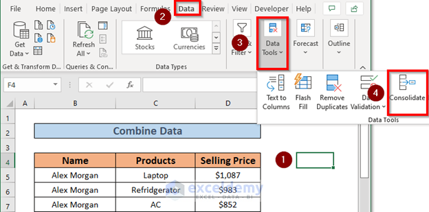
- Select cell F4.
- Go to the Data tab, choose Data tools, and select Consolidate.
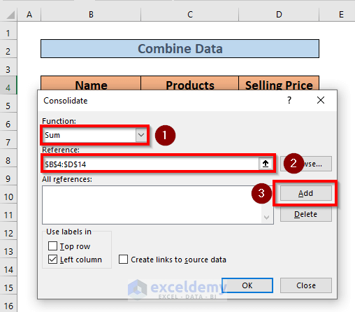
- A Consolidate dialog box will pop up. Set the function to Sum.
- Set the reference to the entire table B4:D14
- Click Add.
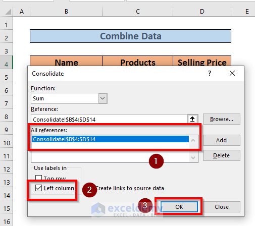
- Mark Left column and click OK.
- Excel will combine the same values and return the sums.
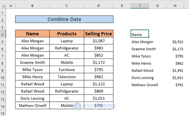
- Format as you wish.
Read More: Concatenate Multiple Cells Based on Criteria in Excel
Method 3 – Applying VBA to Combine Cells with the Same Value
Steps:
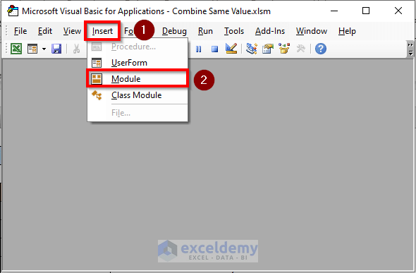
- Press ALT + F11 to open the VBA window.
- Go to Insert and select Module.
- Copy the following code in the Module:
Sub CombineCells()
    Dim Col As New Collection
    Dim Sr As Variant
    Dim Rs() As Variant
    Dim M As Long
    Dim N As Long
    Dim Rg As Range
    Sr = Range("B4", Cells(Rows.Count, "B").End(xlUp)).Resize(, 2)

    Set Rg = Range("E4")
    On Error Resume Next
    For M = 2 To UBound(Sr)
        Col.Add Sr(M, 1), TypeName(Sr(M, 1)) & CStr(Sr(M, 1))
    Next M

    On Error GoTo 0
    ReDim Rs(1 To Col.Count + 1, 1 To 2)

    Rs(1, 1) = "Name"
    Rs(1, 2) = "Products"
    For M = 1 To Col.Count
        Rs(M + 1, 1) = Col(M)
        For N = 2 To UBound(Sr)
            If Sr(N, 1) = Rs(M + 1, 1) Then
                Rs(M + 1, 2) = Rs(M + 1, 2) & ", " & Sr(N, 2)
            End If
        Next N
        Rs(M + 1, 2) = Mid(Rs(M + 1, 2), 2)
    Next M

    Set Rg = Rg.Resize(UBound(Rs, 1), UBound(Rs, 2))
    Rg.NumberFormat = "@"
    Rg = Rs
    Rg.EntireColumn.AutoFit
End Sub
Here, we have created a Sub Procedure “CombineCells”. With the dim statement, we have declared Col, Sr, Rs, M, N, Rg as variables.
The Rg variable is set at E4 which indicates that the result will be displayed at E4.
A For loop will list out the products. We used the Ubound function with Rs as arrayname.
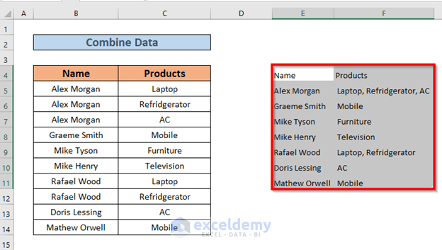
- Press F5 to run the code. Excel will combine the names.
Read More: How to Combine Cells into One with Line Break in Excel
Practice Workbook
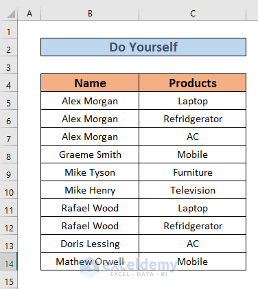
We have attached a practice sheet for you in the sample datasheet.
Download Practice Workbook
Related Articles
- How to Combine Two Cells in Excel with a Dash
- Combine Multiple Cells into One Separated by Comma in Excel
- Concatenate Multiple Cells but Ignore Blanks in Excel
- How to Merge Cells Using Excel Formula
- How to Merge Multiple Cells without Losing Data in Excel
- How to Merge Cells Vertically Without Losing Data in Excel
<< Go Back To Excel Concatenate Multiple Cells | Concatenate Excel | Learn Excel
Get FREE Advanced Excel Exercises with Solutions!

Akib,
I am a neophyte in Excel. I have column A as Ideas then Columns 2 and above I have the category they belong.
Idea/Baby/Infant/Teeen/Young Adult/Adult/etc.
I have X’s in columns B-L. I am listing ideas randomly and wanted to know if there is an easy way to sort by each columns so all my Baby’s/Teen’s etc are together and the ideas are attached to them. Probably easy just not sure how to do it.
Thanks for any pointers or links.
Hello Mr. Clark. Thanks for your valuable comment. In your query, you wanted to know about category-wise idea sorting. If I misunderstood your problem then please let me know about this. I am adding the sorted image here. Then I have described how I have done that.
Firstly, you need to set a list of ideas according to your category just like the image below.
Then in cell B5 write up the following formula.
=IF($B$4=J5,I5,"")Similarly, you have to put the same formula for the other columns but need to set the cell reference for the corresponding cells.
Then drag down the Fill handle Tool for C5, D5, E5 ad F5 cells to get the same formula.
Finally, you will get the result.
Now, if you want to add any category-wise idea then it will automatically be sorted in your dataset list. See the image for a better clarification.