How to Combine Cells into One with Line Break in Excel: 5 Methods

Method 1 – Using the Ampersand Operator and CHAR Function

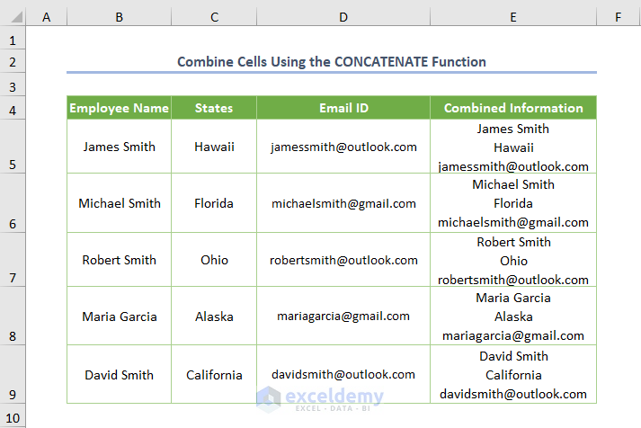
Assuming that you want to get combined information by merging two or more cells. The following example, I am going to find the Combined Information (E5:E9 cell range) covering the information of the previous 3 fields (the Name, States, and Email ID of each employee).

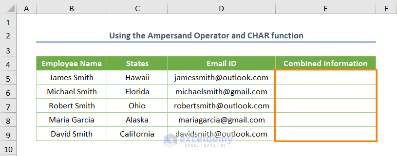
You may extract the output from the different cell ranges by using the ampersand symbol (&) and CHAR function. Insert the following formula in the E5 cell.

B5 is the starting cell of the Employee Name, C5 is the starting cell of the States, and D5 is the starting cell of the Email ID.

In the above formula, the CHAR function checks the character on the basis of a given number or code. The ASCII code for inserting a line break is 10, so we must use CHAR(10) to embed a line break between the combined cells.

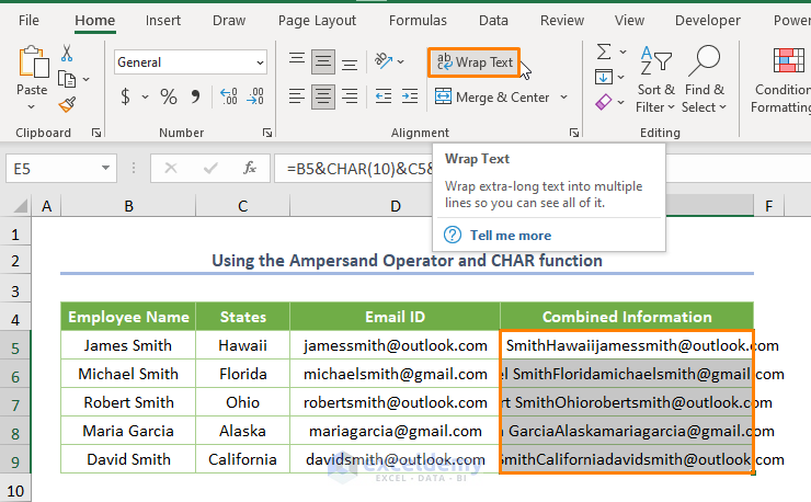
Press ENTER and drag down the plus sign located at the lower-right corner of the E5 cell (Fill Handle Tool). Immediately, you’ll get the output (E5:E9 cell range).

The three cells are combined but you cannot see the output with line break until you turn on the Wrap Text option from the Alignment ribbon in the Home tab. Before doing make sure that you select the output.

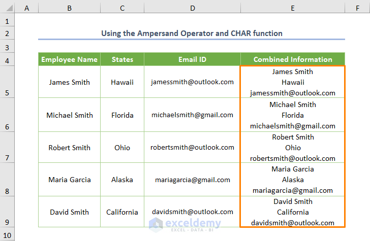
After adjusting the row height, you’ll get the following output, in which the cells are combined, keeping with the line break.

Method 2 – Using the CONCATENATE Function to Combine Cells into One

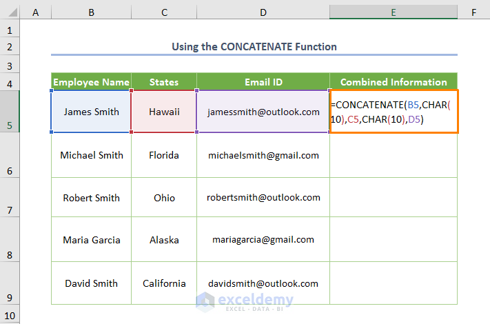
Accomplish the same task using the CONCATENATE function, which combines multiple strings to a single string. The adjusted formula associated with the CHAR function will be-

The ENTER key, use the Fill Handle Tool. The output will look like the following.

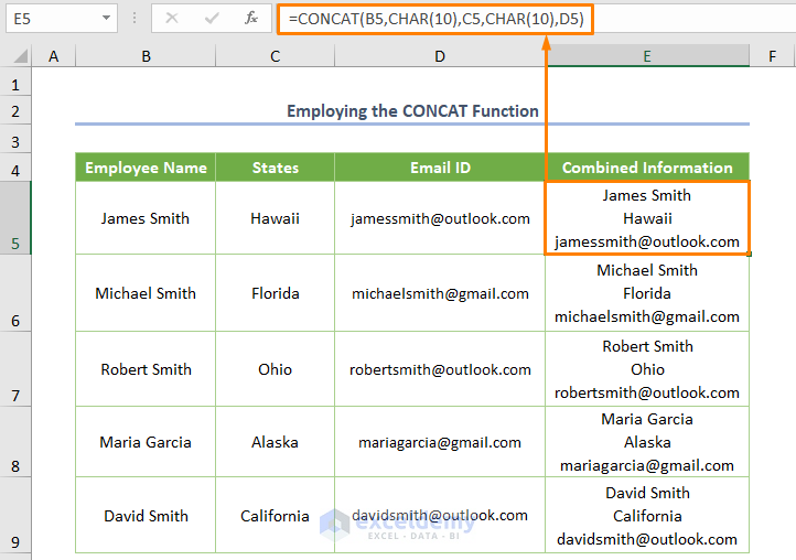
Method 3 – Utilizing the CONCAT Function

You may unify multiple cells into one keeping the line break utilizing the CONCAT. Microsoft recommends the function instead of using the CONCATENATE function. The combined formula for E5 cell will be-

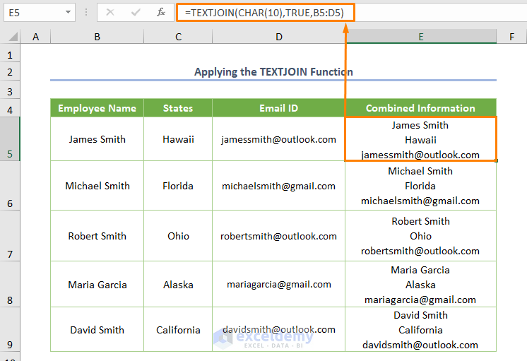
Method 4 – Combine Cells Applying the TEXTJOIN Function with Line Break

If you’re using Microsoft 365 version (any upper versions including Excel 2019), you may apply the TEXTJOIN function. The function joins multiple strings including a delimiter character. Whatever the formula for today’s dataset will be like the following.

B5:D5 is the cell range covering three cells to combine into one. We used TRUE to exclude any empty cells, but if you want to count empty cells, input FALSE.

Method 5 – Combine Cells into One with Line Break Using the VBA Code

Step 01:

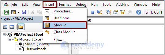
Open a module by clicking Developer > Visual Basic.

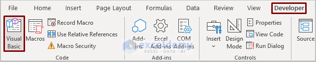
Go to Insert > Module.

Step 02:

Copy the following code.

Sub CombiningCells_VBA()
Range("E5").Value = Range("B5").Value & vbNewLine & Range("C5").Value & vbNewLine & Range("D5").Value
Range("E6").Value = Range("B6").Value & vbNewLine & Range("C6").Value & vbNewLine & Range("D6").Value
Range("E7").Value = Range("B7").Value & vbNewLine & Range("C7").Value & vbNewLine & Range("D7").Value
Range("E8").Value = Range("B8").Value & vbNewLine & Range("C8").Value & vbNewLine & Range("D8").Value
Range("E9").Value = Range("B9").Value & vbNewLine & Range("C9").Value & vbNewLine & Range("D9").Value
End Sub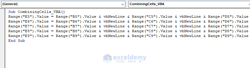

We specified the output cell as the E5 cell with the Range.Value property. The input cells (B5, C5 and D5) are defined. I utilized the Ampersand operator and vb New Line field to combine the multiple cells and keep the line break respectively. We applied the same procedure for the rest of the cells.

Step 03:

Run the code (the keyboard shortcut is F5 or Fn + F5), you’ll see the following output.

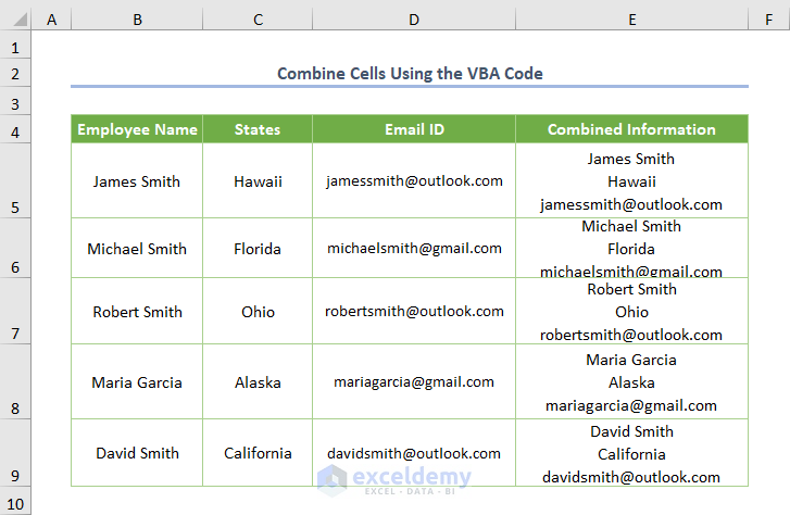
Note: You may also use the vbCrLf and vbLf constants instead of using the vbNewLine.

Things to Remember

• If you want to input an array or cell range, you should use the TEXTJOIN function. Because the CONCATENATE or CONCAT function deals with individual cells.
• Furthermore, you might combine cells into one with a line break separated by a delimiter e.g. comma.

Download Practice Workbook

Related Articles

• How to Combine Cells with Same Value in Excel
• Combine Two Cells in Excel with a Dash
• How to Merge Multiple Cells without Losing Data in Exce
  
• How to Merge Cells Vertically Without Losing Data in Excel

<< Go Back To Excel Concatenate Multiple Cells | Concatenate Excel | Learn Excel