Combine Multiple Cells into One Separated by Comma in Excel

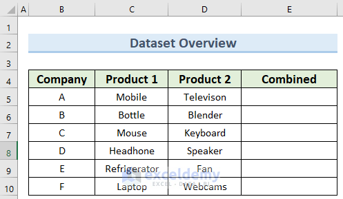
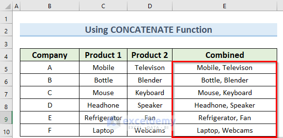
The sample dataset has a listing of products. We’ll combine the products from the two columns into the fourth column, separating the values by a comma.

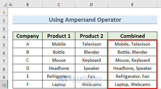
Method 1 – Using the Ampersand Operator to Combine Multiple Cells

Steps:

• Go to cell E5 and insert the following formula:

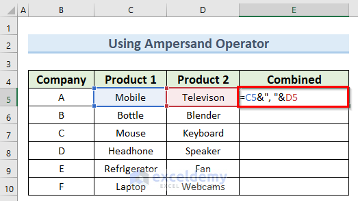
• Press Enter and copy this formula down to the other cells.

Read More: How to Merge Cells Using Excel Formula

Method 2 – Combine Multiple Cells into One with the CONCATENATE Function

Steps:

• Double-click on cell E5 and enter the below formula:

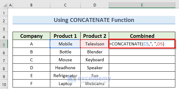
• Press the Enter key and copy this formula down using the Fill Handle.

Read More: How to Combine Cells with Same Value in Excel

Method 3 – Applying the CONCAT Function

Steps:

• Insert the following formula inside cell E5:

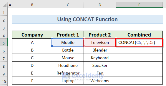
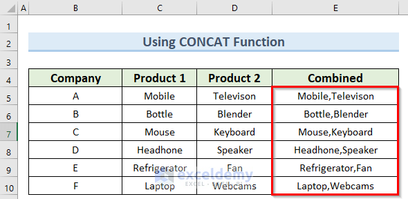
• Press the Enter key.
• AutoFill the formula to the other cells in column E.

Read More: How to Combine Cells into One with Line Break in Excel

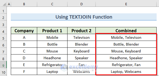
Method 4 – Utilizing the TEXTJOIN Function

Steps:

• Go to cell E5 and insert the following formula:

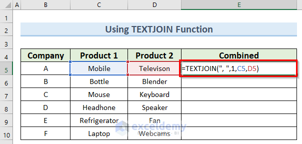
• Hit Enter and copy this formula down by dragging the Fill Handle.

Read More: How to Combine Two Cells in Excel with a Dash

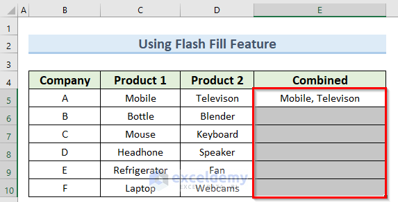
Method 5 – Using Excel Flash Fill to Combine Multiple Cells with a Comma

Steps:

• Type in the expected value (contents of C5, then a comma, then the contents of D5) in cell E5.
• Select all the cells from E5 to E10.

• Click on Flash Fill under the Data Tools group of the Data Tab at the top of the screen.

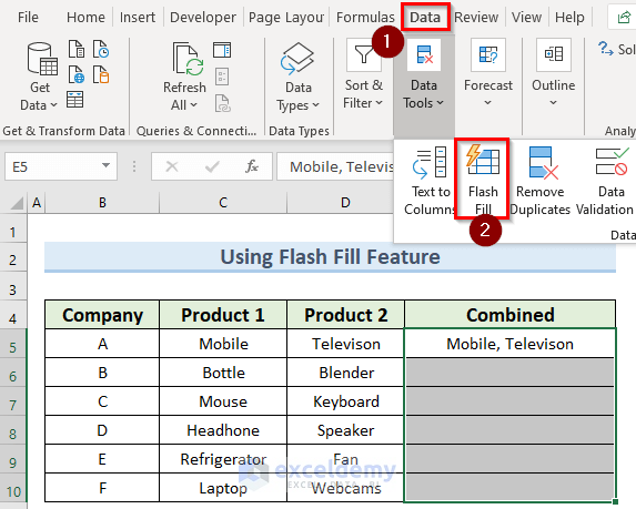
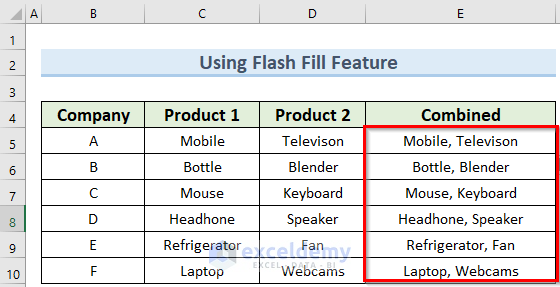
• The Flash Fill feature will identify the pattern of cell E5 and apply it to the other cells.

Read More: How to Merge Multiple Cells without Losing Data in Excel

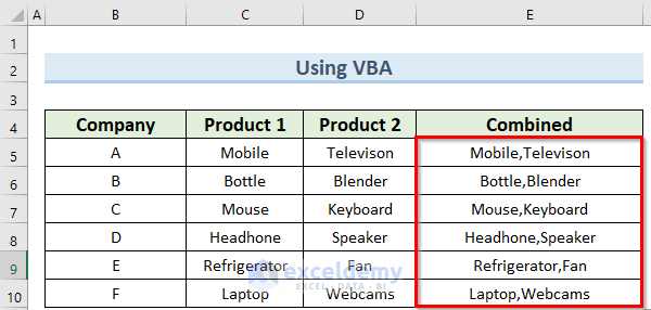
Method 6 – Using VBA to Combine Multiple Cells

Steps:

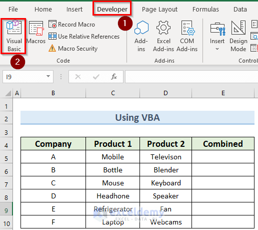
• Go to the Developer tab and select Visual Basic.

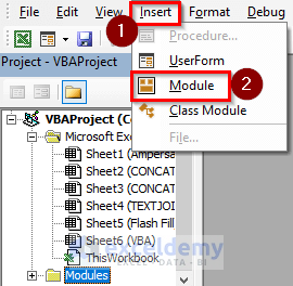
• Select Insert in the VBA window and click on Module.

• Insert the code below in the new window:

Function CombineCells(WorkingRange As Range, Optional Sign As String = ", ") As String
Dim Sh_Rng As Range
Dim ResultStr As String
For Each Sh_Rng In WorkingRange
If Sh_Rng.Value <> " " Then
ResultStr = ResultStr & Sh_Rng.Value & Sign
End If
Next
CombineCells = Left(ResultStr, Len(ResultStr) - Len(Sign))
End Function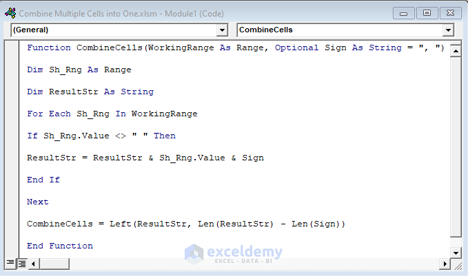

• Save the file.
• Go to cell E5 and insert the following formula:

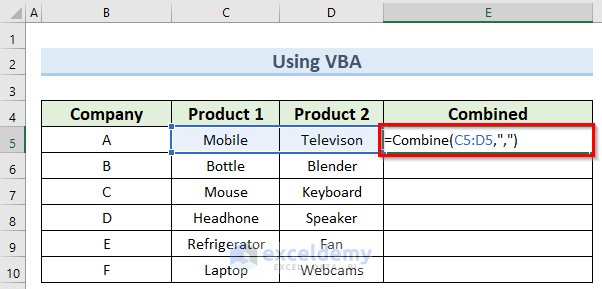
• Press the Enter key and use the Fill Handle.

Read More: How to Merge Cells Vertically Without Losing Data in Excel

Download the Practice Workbook

Further Readings

• How to Concatenate Multiple Cells in Excel
• Concatenate Multiple Cells Based on Criteria in Excel
• Concatenate Multiple Cells but Ignore Blanks in Excel

<< Go Back To Excel Concatenate Multiple Cells | Concatenate Excel | Learn Excel