Concatenate Multiple Cells Based on Criteria in Excel (4 Methods)

Here’s an overview of concatenating cells if they meet certain criteria.

How to Concatenate Multiple Cells Based on Criteria in Excel: 4 Easy Ways

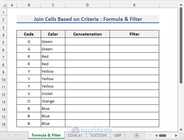
Method 1 – Combine Multiple Cells Based on Criteria with Formula and a Filter

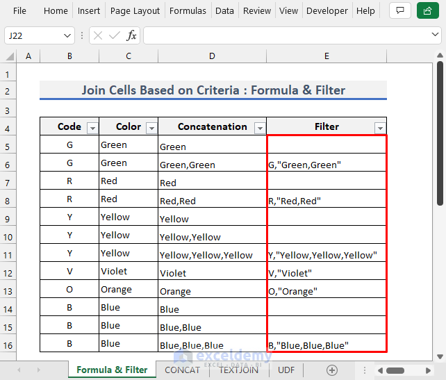
We have the following dataset containing colors with codes. We’ll concatenate the Color cells based on their codes.

Steps

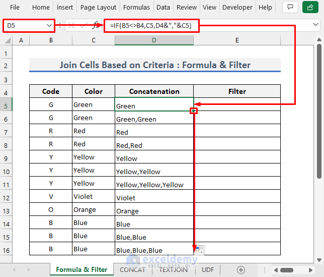
• Enter the following formula in cell D5:

• Use the fill handle tool to apply this formula to the cells below.

• Apply the following formula in cell E5:

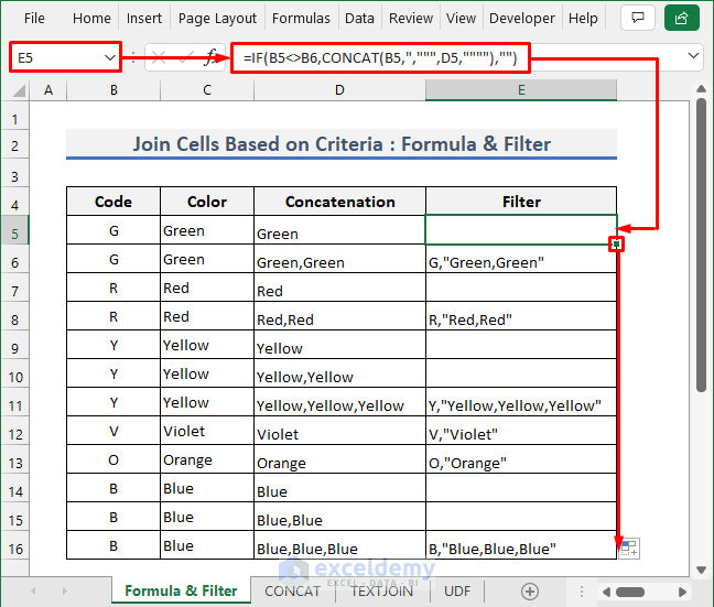
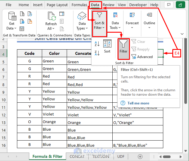
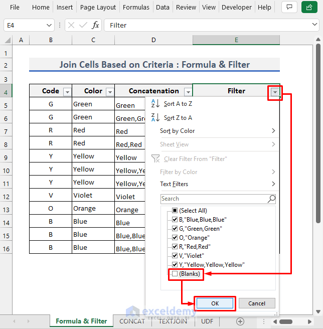
• Select cell E4.
• Select Sort & Filter and choose Filter from the Data tab as shown in the following picture.

• The Filter column will look as follows.

• Click on the drop-down arrow in cell E4.
• Uncheck (Blanks).
• Click OK.

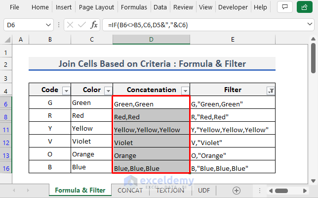
• The Color cells will be concatenated as follows.

Read More: Concatenate Multiple Cells but Ignore Blanks in Excel

Method 2 – Concatenate Multiple Cells Based on Criteria with the CONCAT Function

Steps

• Modify the earlier dataset as follows.

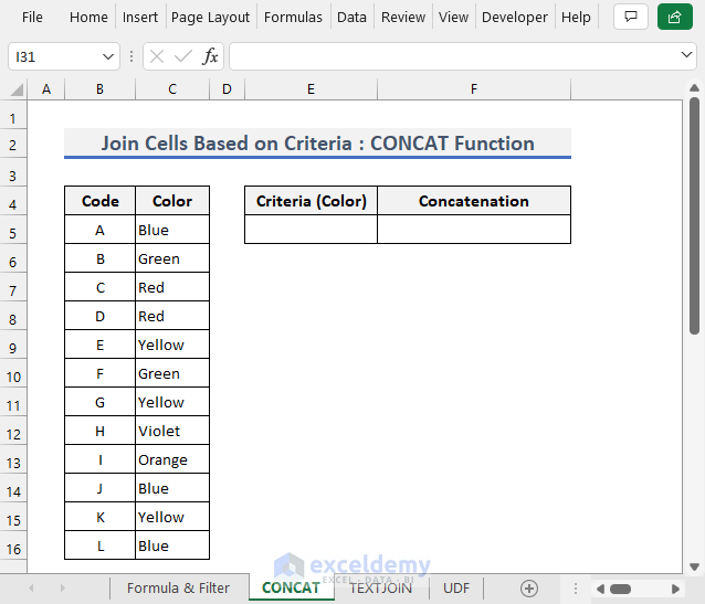
• Enter the following formula in cell F5:

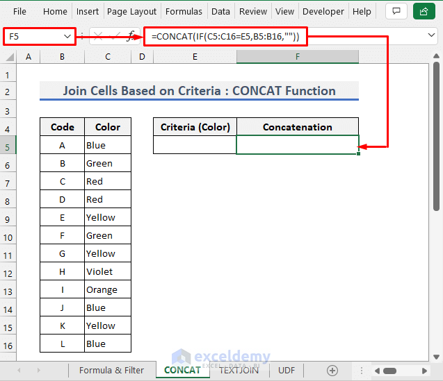
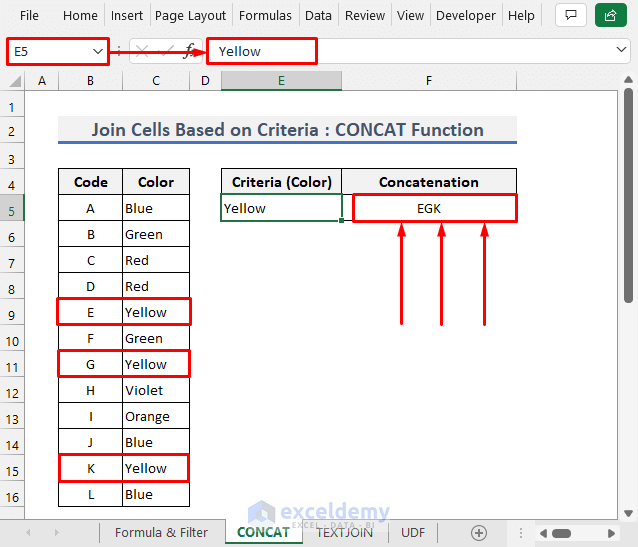
• Enter a color name in cell E5. We put Yellow for the example.
• The result will look as follows.

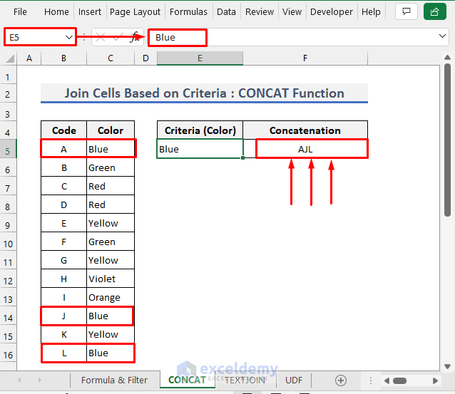
• Change the Color name and see how the result changes.

Read More: How to Concatenate Multiple Cells in Excel

Method 3 – Join Multiple Cells Based on Criteria with the TEXTJOIN Function

Steps

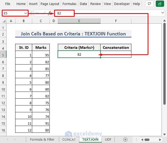
• We have a dataset with Student IDs and Marks.

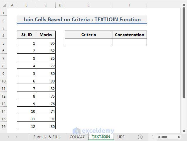
• We want the student IDs for those who got more marks than the criteria (E5) concatenated in cell F5.
• Enter the criteria in cell E5.

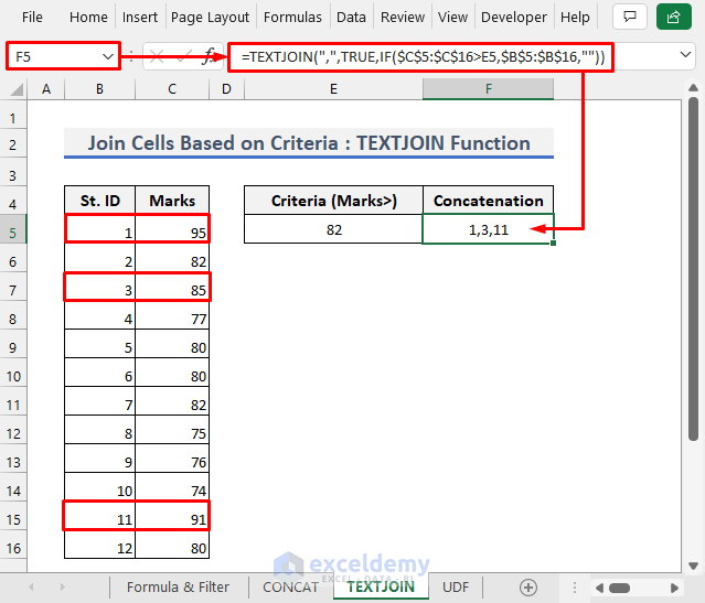
• Apply the following formula in cell F5.

• You will see the IDs concatenated as follows.

• You can change the criteria value as well as the criteria in the formula.
• To find student IDs for students who got equal to or lower marks than the condition, use:

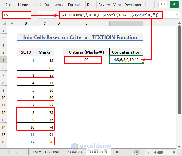
Read More: Combine Multiple Cells into One Separated by Comma in Excel

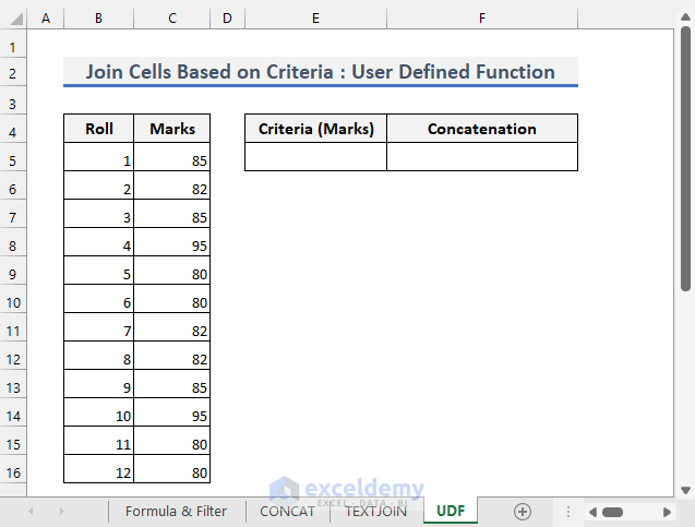
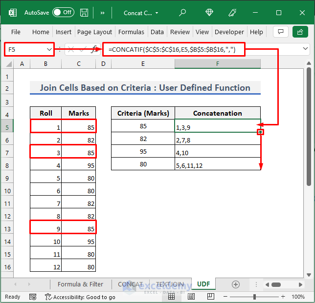
Method 4 – Concatenate Multiple Cells Based on Criteria with a UDF

Steps

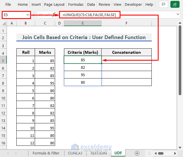
• Consider the following dataset similar to the earlier one.

• Enter the following formula in cell E5.

• This gives the list of unique marks obtained by the students.

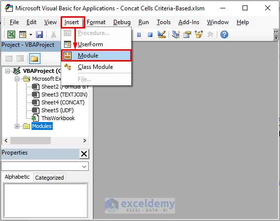
• Press Alt + F11 to open the Microsoft Visual Basic for Applications. You will also find it in the Developer tab.
• Select Insert and choose Module.

• Copy the following code and paste it on the blank module.

Function CONCATIF(Criteria As Range, Concatcriteria As Variant, ConcatRange As Range, Optional Delimiter As String = ",") As Variant
Dim Results As String
On Error Resume Next
If Criteria.Count <> ConcatRange.Count Then
    CONCATIF = CVErr(xlErrRef)
    Exit Function
End If
For j = 1 To Criteria.Count
    If Criteria.Cells(j).Value = Concatcriteria Then
        Results = Results & Delimiter & ConcatRange.Cells(j).Value
    End If
Next j
If Results <> "" Then
    Results = VBA.Mid(Results, VBA.Len(Delimiter) + 1)
End If
CONCATIF = Results
Exit Function
End Function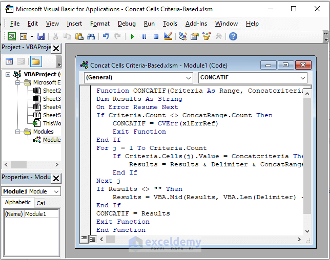

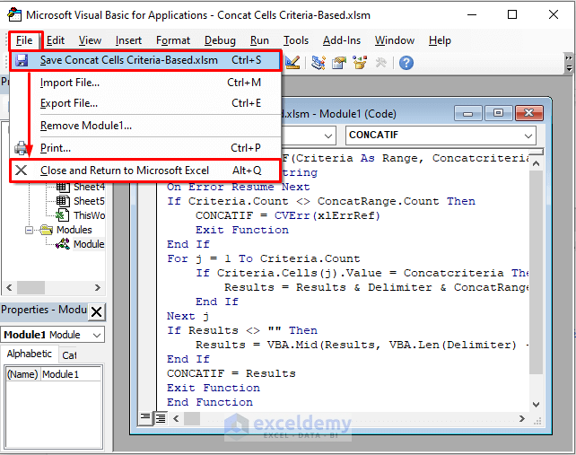
• Select Close and Return to Microsoft Excel from the File tab.

• Apply the following formula in cell F5 and drag it to the cells below.

• You will see the result as follows.

Read More: How to Merge Cells Using Excel Formula

Things to Remember

• The CONCATENATE function is an earlier version to the CONCAT function. Both functions give the same result.
• The TEXTJOIN function may only be available in the newer versions of Microsoft Excel.

Download the Practice Workbook

Related Articles

• How to Combine Cells with Same Value in Excel
• How to Combine Cells into One with Line Break in Excel
• How to Combine Two Cells in Excel with a Dash
• How to Merge Multiple Cells without Losing Data in Excel
• How to Merge Cells Vertically Without Losing Data in Excel

<< Go Back To Excel Concatenate Multiple Cells | Concatenate Excel | Learn Excel